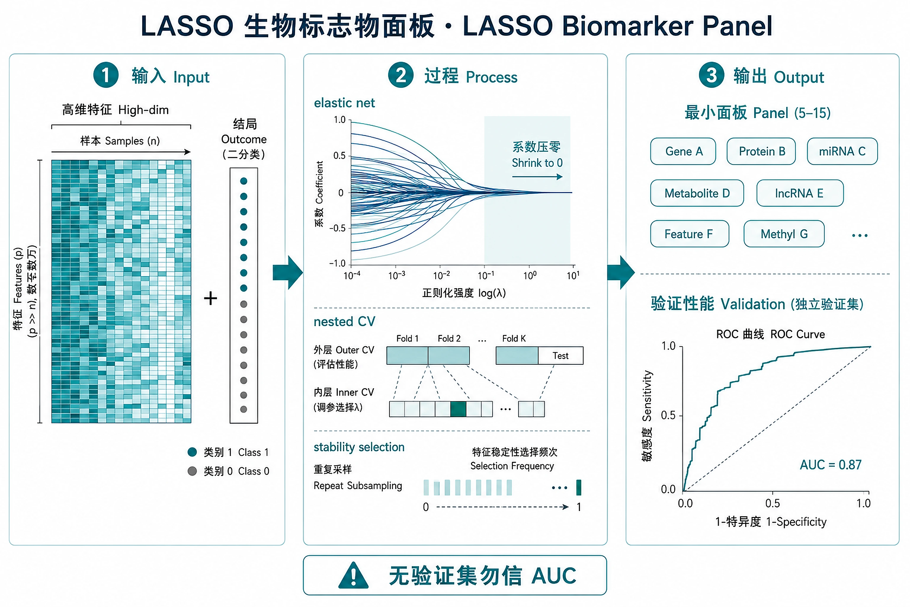
LASSO Biomarker Panel
A minimal 5–15 feature panel via LASSO.
Overview
Problem. Which few features predict the outcome stably?
Learning goals
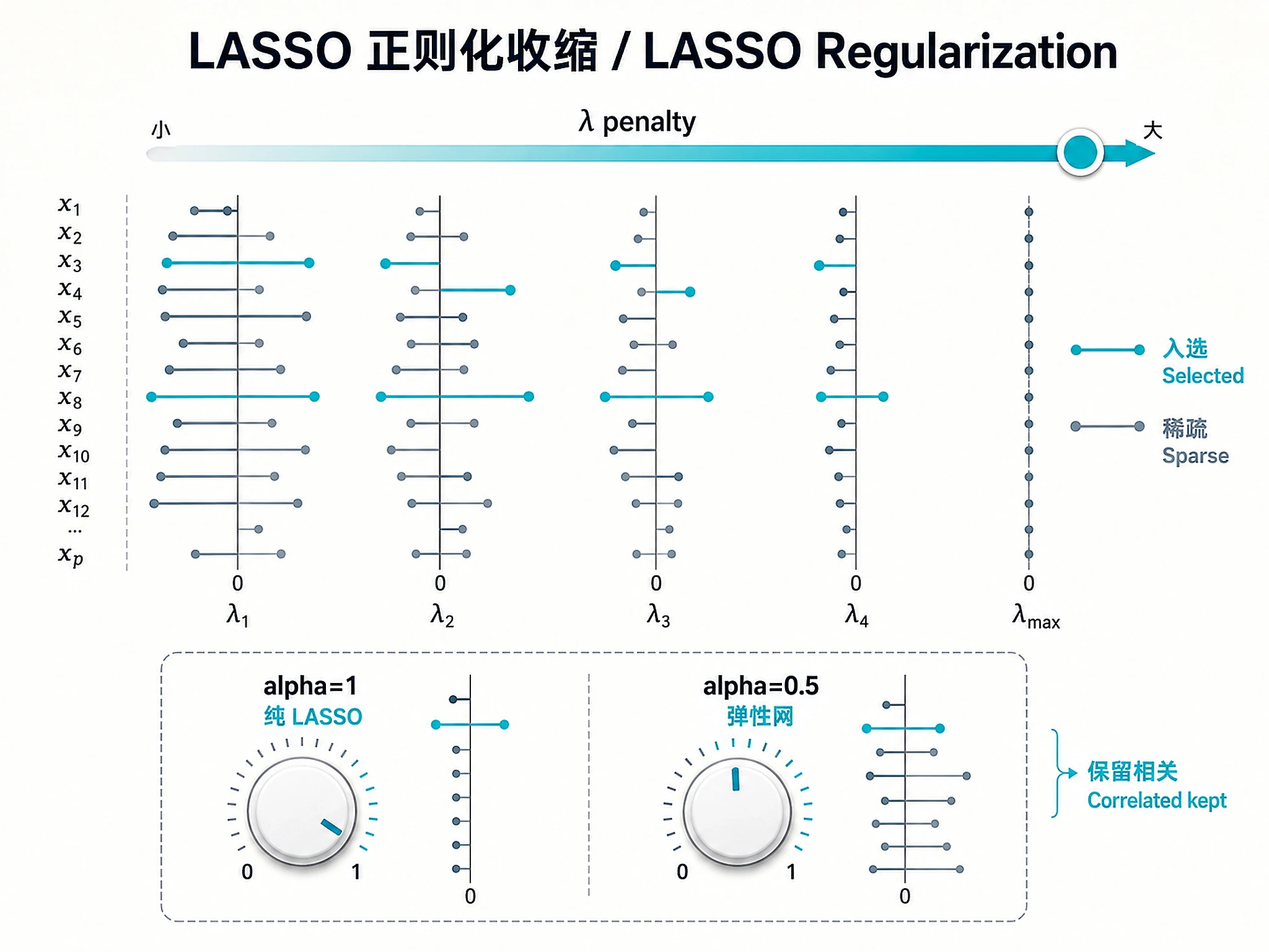
- Regularisation zeroes out weak features
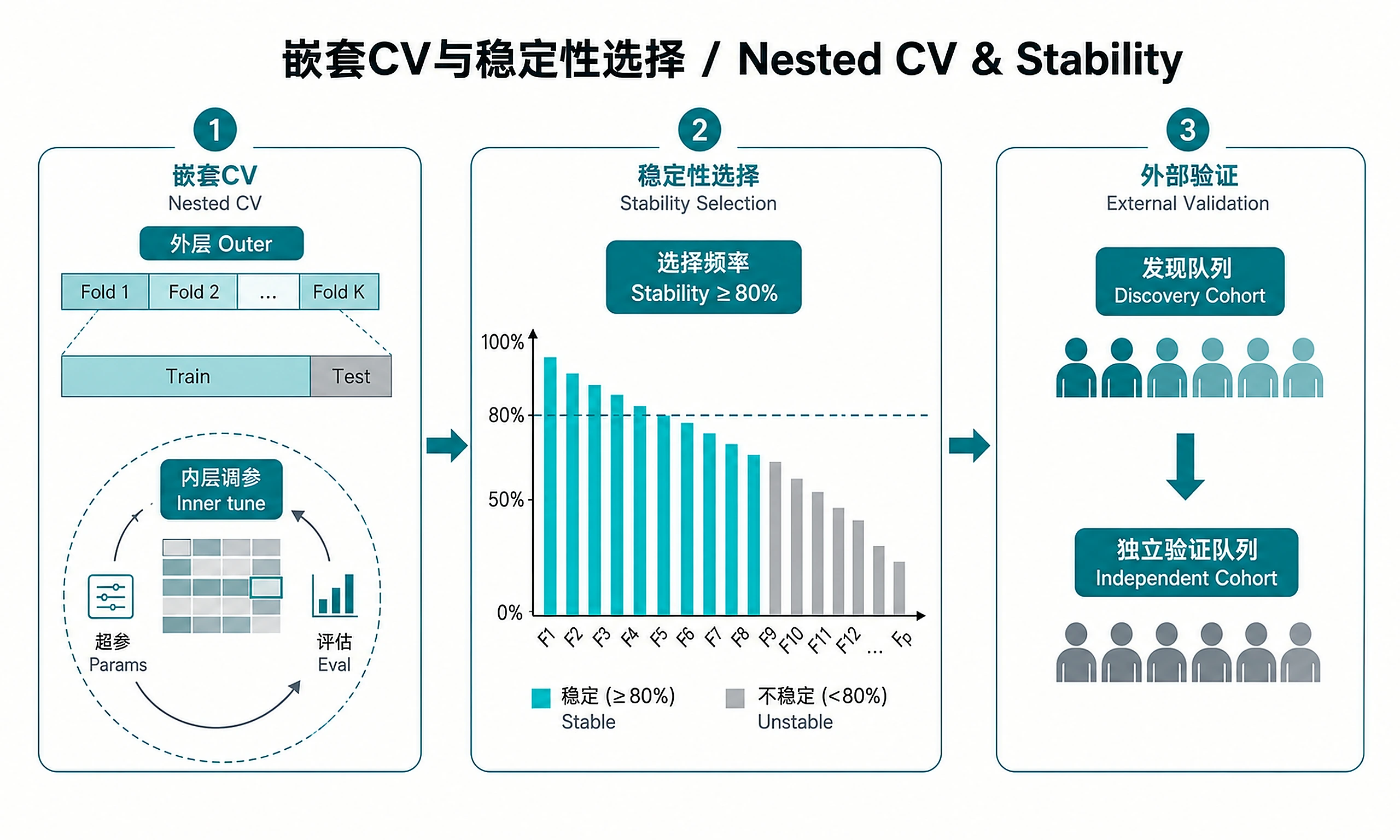
- Nested CV prevents leakage and inflated AUC
Figures
Tutorial
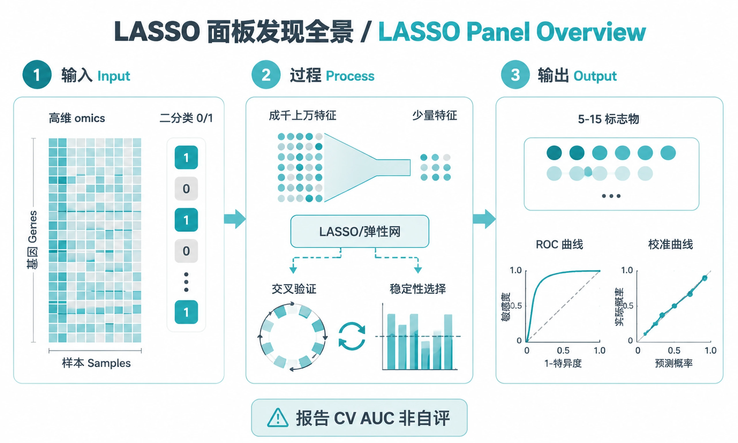
Select minimal, interpretable biomarker panels from high-dimensional omics data using penalized logistic regression (LASSO/elastic net) with nested cross-validation and stability selection.
When to Use This Skill
Use this skill when you need to:
- Select a minimal biomarker panel (5-15 features) from thousands of candidates
- Build a predictive model for a binary clinical outcome (responder/non-responder, disease/control)
- Validate across cohorts — discovery + independent validation design
- Generate regulatory-grade outputs — ROC/AUC, calibration, decision curves
- Design clinical exploratory endpoints from omics biomarker signatures
Don't use this skill for:
- Unsupervised clustering (use
bulk-omics-clustering) - Differential expression only (use
bulk-rnaseq-counts-to-de-deseq2) - Multi-omics integration/factor discovery (use
multiomics-patient-stratification) - Continuous outcomes — this skill is for binary classification
Installation
options(repos = c(CRAN = "https://cloud.r-project.org"))
if (!require('BiocManager', quietly = TRUE)) install.packages('BiocManager')

# Core (required)
install.packages(c('glmnet', 'pROC', 'ggplot2', 'ggprism', 'ggrepel'))

# Heatmap (required for feature heatmap)
BiocManager::install(c('ComplexHeatmap'))
install.packages('circlize')

# Example data — Sepsis MARS consortium (recommended demo) + breast cancer/UNIFI
BiocManager::install(c('GEOquery', 'Biobase'))

# Example data — IMvigor210 bladder cancer IO (alternative demo)
install.packages('remotes')
remotes::install_github('SiYangming/DESeq', upgrade = 'never')
remotes::install_github('SiYangming/IMvigor210CoreBiologies', upgrade = 'never')
BiocManager::install('DESeq2')

# Optional: DE pre-filtering
BiocManager::install('limma')

# Optional: Biological interpretation (pathway enrichment, cell-type context)
BiocManager::install(c('clusterProfiler', 'org.Hs.eg.db', 'fgsea'))
install.packages('msigdbr')
| Software | Version | License | Commercial Use | Installation |
|---|---|---|---|---|
| glmnet | >=4.1 | GPL-2 | Permitted | install.packages('glmnet') |
| pROC | >=1.18 | GPL (>=3) | Permitted | install.packages('pROC') |
| ggplot2 | >=3.4 | MIT | Permitted | install.packages('ggplot2') |
| ggprism | >=1.0.3 | GPL (>=3) | Permitted | install.packages('ggprism') |
| ggrepel | >=0.9 | GPL-3 | Permitted | install.packages('ggrepel') |
| ComplexHeatmap | >=2.10 | MIT | Permitted | BiocManager::install('ComplexHeatmap') |
| circlize | >=0.4.15 | MIT | Permitted | install.packages('circlize') |
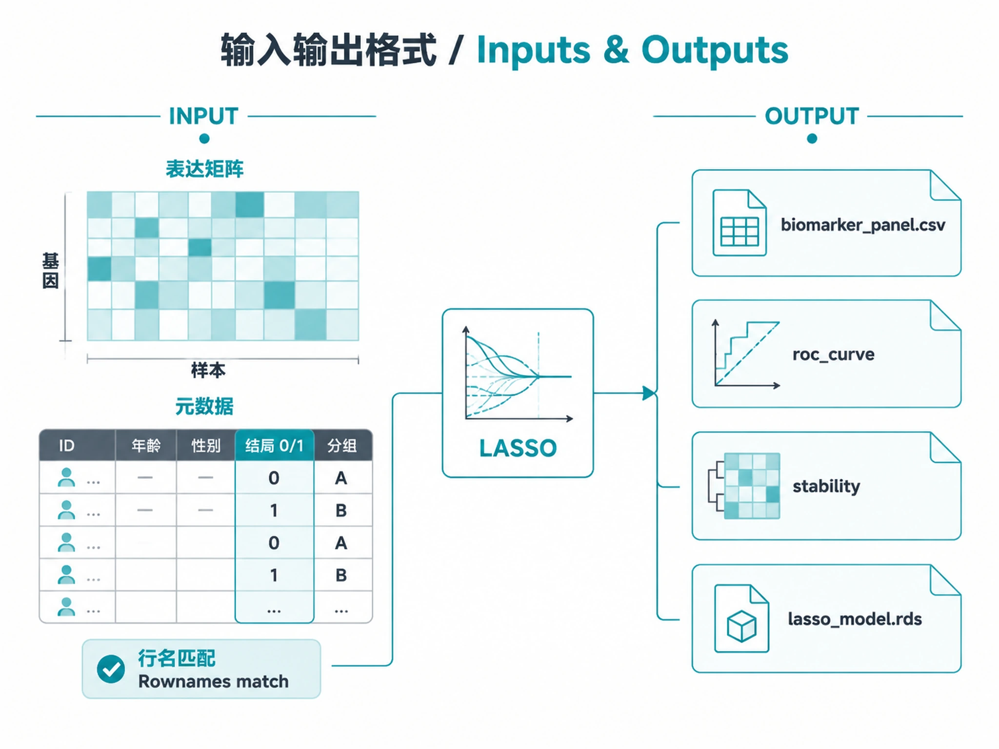
Inputs
Required:
- Expression matrix (genes x samples): TPM, FPKM, normalized counts, or protein abundance
- Sample metadata: Data frame with a binary outcome column (0/1 or two-level factor)
- Rownames must match expression column names
- Minimum 20 samples per group (40+ recommended)
Optional:
- Validation cohort: Independent expression matrix + metadata with same outcome
- Pre-filtered feature list: From DE analysis or WGCNA hub genes (see Related Skills)
Outputs
Primary results:
biomarker_panel.csv— Final panel features with LASSO coefficients and selection frequenciesall_feature_stability.csv— All features ranked by selection frequencydiscovery_performance.csv— Per-fold AUC, sensitivity, specificityvalidation_performance.csv— External validation metrics (if validation cohort provided)
Analysis objects (RDS):
lasso_model.rds— Complete model result for downstream use- Load with:
model <- readRDS('results/lasso_model.rds') - Predict with:
source("scripts/lasso_workflow.R"); predict_biomarker_panel(model, new_X) - Required for:
multiomics-patient-stratification, downstream prediction
Plots (PNG + SVG at 300 DPI):
roc_curve.png/.svg— ROC curve (discovery + validation overlay)stability_barplot.png/.svg— Feature selection frequency across CV foldscoefficient_forest.png/.svg— LASSO coefficients with 95% CIscalibration_curve.png/.svg— Predicted vs observed probabilityauc_distribution.png/.svg— AUC distribution across CV foldsfeature_heatmap.png/.svg— Clustered heatmap of panel features
Reports:
summary_report.md— Comprehensive analysis report (goals, context, datasets, methods, results)summary_report.pdf— PDF report (only if tinytex installed; falls back to HTML automatically — this is expected in most environments)summary_report.Rmd— R Markdown source (customizable)
Clarification Questions
ALWAYS ask Question 1 FIRST.
1. Example or Own Data? (ASK THIS FIRST):
- a) Run example dataset to showcase the workflow (recommended)
- Runs a sepsis blood transcriptomics demo (MARS Consortium, ICU patients) that derives a ~15–25 gene panel for identifying immunosuppressed sepsis patients — CV AUC ~0.986 (discovery cohort estimate; panel size varies across runs)
- No further questions needed. Proceed directly to Step 1 with all defaults.
- b) I have my own expression data and patient outcomes to analyze
- Continue to Questions 2-4 below
IF EXAMPLE SELECTED (option a): Skip all remaining questions. Run Step 1 with:
data <- load_sepsis_data(outcome = "endotype"), then Steps 2-4 with defaults (top_n_variable = 2000,alpha = 0.5,disease = "sepsis").
Questions 2-4 are ONLY asked if the user selected option (b) — own data:
2. Input Files (own data only):
- What expression data file(s) do you have? (CSV, TSV, RDS, or Bioconductor object)
- Expected: Gene/protein × sample matrix (rows = features, columns = samples)
- What metadata/clinical file do you have?
- Must include a binary outcome column (0/1 or two-level factor)
- Rownames must match expression column names
3. Outcome & Organism (own data only):
- What is the binary outcome column name in your metadata?
- What do the two levels represent? (e.g., responder/non-responder, disease/control)
- What organism? (human/mouse/rat — for pathway enrichment)
4. Analysis Options (own data only — structured):
- LASSO regularization:
- a) Pure LASSO, alpha=1.0 (sparsest panel)
- b) Elastic net, alpha=0.5 (recommended — retains correlated features)
- Feature pre-filtering:
- a) Top 2000 most variable features (recommended for >5000 features)
- b) Top 500 most variable (for smaller datasets or faster runs)
- c) Use all features (no filtering)
Standard Workflow
MANDATORY: USE SCRIPTS EXACTLY AS SHOWN - DO NOT WRITE INLINE CODE
Step 1 - Load data:
source("scripts/load_example_data.R")
data <- load_sepsis_data(outcome = "endotype")  # 479 ICU patients, Mars1 endotype classification
# OR: data <- load_sepsis_data(outcome = "mortality")  # 479 patients, 28-day mortality
# OR: data <- load_breast_cancer_pcr_data(outcome = "subtype")  # 218 tumors, Basal vs LumA
# OR: data <- load_imvigor210_data()   # 190 bladder cancer patients, atezolizumab
# OR: data <- load_unifi_data()        # 542 UC patients, UNIFI ustekinumab trial
DO NOT write custom data loading code. Use the loader functions.
✅ VERIFICATION: You MUST see: "✓ Sepsis endotype data loaded successfully!" (or similar per dataset)
Step 2 - Run LASSO analysis:
source("scripts/prepare_features.R")
features <- prepare_feature_matrix(data$expression, data$metadata, data$outcome_col, top_n_variable = 2000)

source("scripts/lasso_workflow.R")
model <- run_lasso_panel(features$X, features$y, alpha = 0.5)
DO NOT write inline LASSO code (glmnet, cv.glmnet, etc.). Just use the scripts.
✅ VERIFICATION: You MUST see: "✓ LASSO panel selection completed successfully!"
IF YOU DON'T SEE THIS: You wrote inline code. Stop and use source().
Step 3 - Generate visualizations:
source("scripts/biomarker_plots.R")
generate_all_plots(model, X = features$X, y = features$y, output_dir = "results")
DO NOT write inline plotting code (ggsave, ggplot, etc.). Just use generate_all_plots().
The script handles PNG + SVG export with graceful fallback for SVG dependencies.
✅ VERIFICATION: You MUST see: "✓ All biomarker plots generated successfully!"
Step 4 - Export results:
source("scripts/export_results.R")
export_all(model, output_dir = "results", data = data, features = features)
DO NOT write custom export code. Use export_all().
Pass data and features for a comprehensive report with disease context and methods.
✅ VERIFICATION: You MUST see: "=== Export Complete ==="
NOTE on PDF: If export_all() reports "PDF rendering failed", this is expected in environments without LaTeX. Inform the user that summary_report.html and summary_report.md are available instead. Do NOT silently omit this from the summary.
⚠️ CRITICAL: Do NOT interpret panel biology without running enrichment
After identifying the panel, do NOT describe gene functions or pathway membership from gene names alone. This is a hallucination risk. Instead:
- State the panel genes and their coefficients/stability scores
- Direct the user to run pathway enrichment as a next step
- Only describe biology if
functional-enrichment-from-degshas been run in this session
✅ Acceptable: "ACSL6 was selected in 100% of folds with a positive coefficient." ❌ NOT acceptable: "ACSL6 is involved in mitochondrial fatty acid metabolism, consistent with..."
Step 5 (Strongly Recommended) — External Validation:
Without this step, all performance metrics are discovery-cohort estimates only and are expected to be optimistic. Do not present results as a validated panel without completing this step.
source("scripts/load_example_data.R")
val_data <- load_breast_cancer_validation_data("GSE32646")  # or load_pursuit_data()
source("scripts/validate_external.R")
source("scripts/prepare_features.R")
val_features <- prepare_validation_features(val_data$expression, features$feature_names)
val_result <- validate_panel(model, val_features$X, val_data$metadata[[val_data$outcome_col]],
                              cohort_name = "GSE32646")
export_all(model, validation_result = val_result, output_dir = "results",
           data = data, features = features)
CRITICAL - DO NOT:
- Write inline LASSO code -> STOP: Use
source("scripts/lasso_workflow.R") - Write inline plotting code -> STOP: Use
generate_all_plots() - Write custom export code -> STOP: Use
export_all() - Try to install svglite -> script handles SVG fallback automatically
IF SCRIPTS FAIL - Script Failure Hierarchy:
- Fix and Retry (90%) - Install missing package, re-run script
- Modify Script (5%) - Edit the script file itself, document changes
- Use as Reference (4%) - Read script, adapt approach, cite source
- Write from Scratch (1%) - Only if genuinely impossible, explain why
NEVER skip directly to writing inline code without trying the script first.
Common Issues
| Error | Cause | Fix |
|---|---|---|
| "No shared samples" | Column names don't match rownames | Check colnames(expression) match rownames(metadata) |
| "Outcome must be binary" | Non-binary outcome column | Ensure 2 unique values in outcome. Recode if multi-level. |
| cv.glmnet convergence warning | Too few samples for 10-fold CV | Reduce n_inner_folds to 5 or increase sample size |
| "No features passed stability" | Very noisy data or small effect | Script auto-relaxes to top 10 features. Consider alpha=0.5 (elastic net). |
| Low validation AUC | Cross-platform gene loss | Check val_features$n_matched. If <50% matched, use same-platform validation. |
| SVG export error | Missing optional dependency | Normal - generate_all_plots() falls back to base R svg() automatically. |
| GEOquery download fails | Network/firewall issue | Retry or download manually from NCBI GEO website |
| PDF report not generated | tinytex/LaTeX not installed | Normal fallback — use summary_report.html or summary_report.md instead. Do NOT silently omit this from the summary. |
Agent Summary Guidelines
When presenting final results to the user, the agent MUST:
- Always cite the CV AUC (from
discovery_performance.csv), never the final model AUC from the ROC plot - Always state whether external validation was performed. If not, include this sentence verbatim:
"These results are from the discovery cohort only. No external validation was performed. AUC estimates are expected to be optimistic."
- Never describe panel gene biology unless
functional-enrichment-from-degswas run in this session - Always report PDF status — if PDF generation failed, say so explicitly and note that .html/.md reports are available
- Never use the word "validated" to describe a panel that has only been tested in the discovery cohort
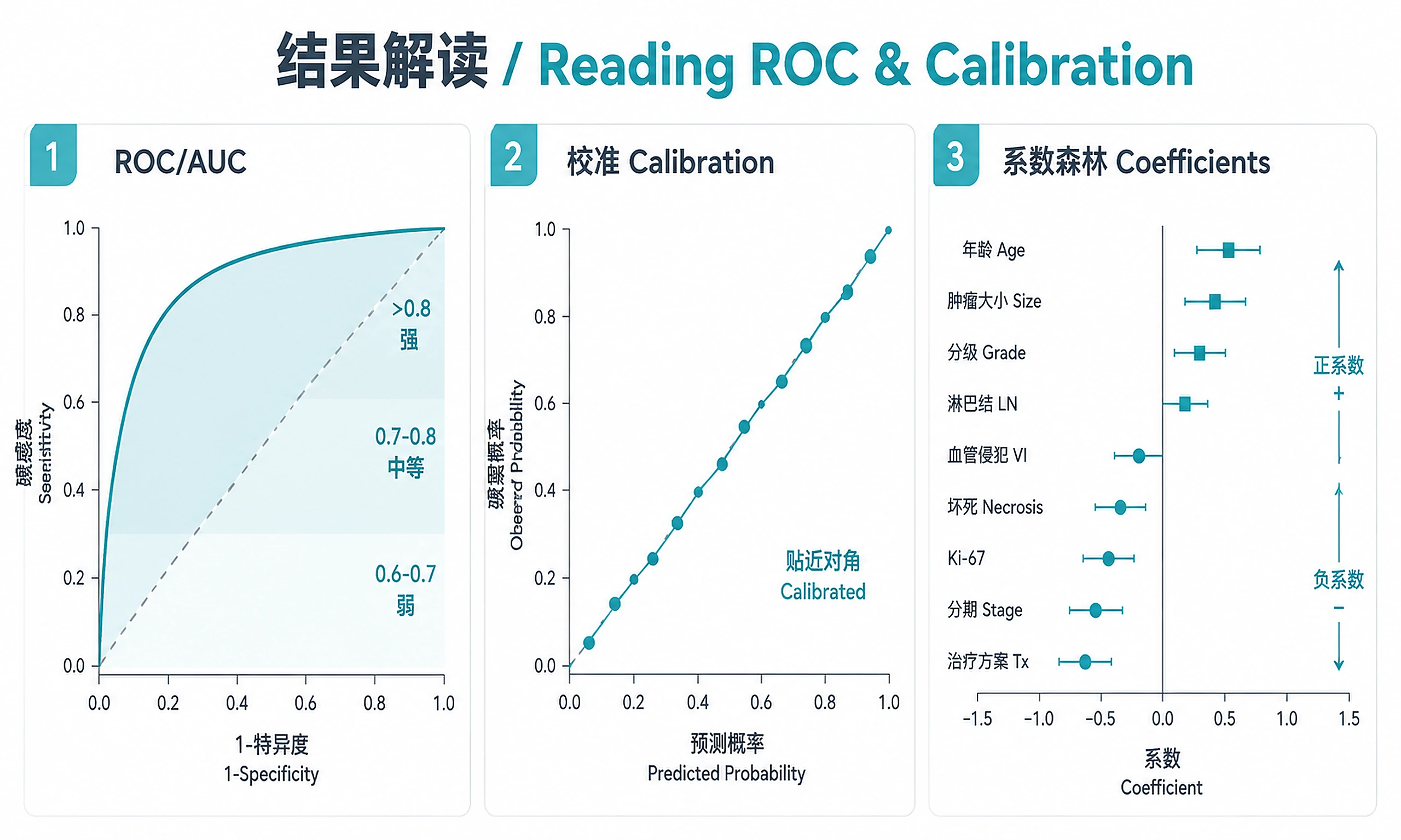
Interpretation Guidelines
- AUC > 0.8: Strong discriminative ability (clinically useful)
- AUC 0.7-0.8: Moderate — useful with other clinical factors
- AUC 0.6-0.7: Weak but above chance — typical for baseline transcriptomic prediction of treatment response
- Stability >= 80%: Feature is robustly selected (high confidence in panel)
- Positive coefficient: Higher expression -> higher probability of positive outcome
- Negative coefficient: Higher expression -> lower probability of positive outcome
- Calibration: Points near diagonal = well-calibrated model
AUC Values — Which Number to Use
Two AUC figures are produced by this workflow:
| Figure | Value | What it means | Use this? |
|---|---|---|---|
Mean CV AUC (discovery_performance.csv) |
e.g. 0.986 | Average AUC across held-out test sets | YES — cite this |
| Final model AUC (ROC curve plot annotation) | e.g. 0.996 | Model applied back to its own training data | NO — in-sample, optimistic |
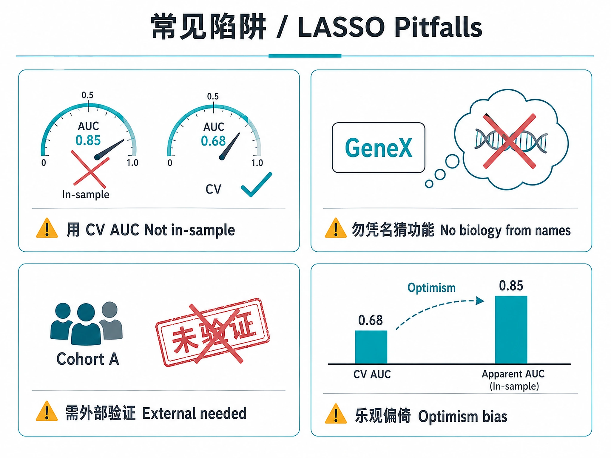
Always report the mean CV AUC as the performance estimate. The final model AUC is only shown for reference and will always be higher.
Interpreting CV AUC: Known Optimism Bias
The reported CV AUC from this workflow is an estimate within the discovery cohort, not a true out-of-sample performance figure. It is subject to optimism bias because:
- Feature stability is computed across the same samples used for AUC estimation
- The final model is re-fit on all samples after feature selection
Expected magnitude of bias: Typically 0.02–0.05 AUC units for datasets of this size. A discovery AUC of 0.986 should be interpreted as "likely >0.93 in an independent cohort if the signal is real" — not as a guaranteed performance floor.
The only way to get an unbiased estimate is external validation.
Suggested Next Steps
After building a biomarker panel:
- [REQUIRED before biological interpretation] Pathway enrichment of panel genes ->
functional-enrichment-from-degs - Co-expression context — which WGCNA modules contain panel genes ->
coexpression-network - Patient stratification using panel as input ->
multiomics-patient-stratification - Literature validation — are panel genes known disease/therapy markers?
- Independent cohort replication on external validation datasets
Related Skills
| Skill | Relationship |
|---|---|
bulk-rnaseq-counts-to-de-deseq2 |
Upstream — DE results can pre-filter features for LASSO |
coexpression-network |
Upstream — WGCNA hub genes as LASSO candidates (Paper 1 cascade) |
functional-enrichment-from-degs |
Downstream — Pathway enrichment of panel genes |
bulk-omics-clustering |
Alternative — Unsupervised patient stratification |
multiomics-patient-stratification |
Downstream — Multi-omics integration + subtyping |
References
- Ali et al., Nature Medicine 2025 — Cross-disease LASSO proteomics panels (AUC 0.81-0.88). Code: github.com/NeuroGenomicsAndInformatics/NatMed_2025_GNPC
- Shen et al., Cell 2024 — WGCNA -> LASSO 6-protein panel (AUC 0.911)
- Sands et al., NEJM 2019 — UNIFI Trial (GSE206285 source)
- Sandborn et al., Gastro 2014 — PURSUIT Trial (GSE92415 source)
- glmnet vignette — Friedman, Hastie, Tibshirani
- pROC package — Robin et al., BMC Bioinformatics 2011
- See references/lasso-reference.md for parameter tuning guide
- See references/validation-guide.md for multi-cohort design
Code preview
scripts/biological_interpretation.R
# Biological Interpretation of Biomarker Panel
#
# Three complementary analyses:
#   1. Pathway enrichment (ORA on panel genes + GSEA on ranked features)
#   2. Cell-type expression context (CZI CELLxGENE Census)
#   3. GWAS genetic risk / disease gene overlap
#
# Usage:
#   source("scripts/biological_interpretation.R")
#   interp <- run_biological_interpretation(model, features, output_dir = "results",
#                                            disease = "ibd")  # or "bladder_cancer", "breast_cancer", or "sepsis"

cat("Loading biological interpretation functions...\n")

# ============================================================
# 1. Pathway Enrichment
# ============================================================

.run_pathway_enrichment <- function(model_result, features = NULL, output_dir = "results") {
    cat("\n--- Pathway Enrichment Analysis ---\n\n")

    suppressPackageStartupMessages({
        library(clusterProfiler)
        library(org.Hs.eg.db)
        library(fgsea)
        library(msigdbr)
        library(ggplot2)
        library(ggprism)
    })

    panel_genes <- model_result$stable_features
    fi <- model_result$feature_importance

    results <- list(ora_go = NULL, ora_kegg = NULL, gsea_hallmark = NULL,
                    gsea_reactome = NULL, gsea_immunologic = NULL)

    # ---- ORA on panel genes (GO:BP) ----
    cat("  ORA: GO Biological Process on", length(panel_genes), "panel genes...\n")

    # Filter out non-standard gene symbols (IGLV4-60 etc.)
    valid_genes <- panel_genes[!grepl("^IGH|^IGK|^IGL|^LOC|^C\\d+orf", panel_genes)]
    cat("    Valid gene symbols for ORA:", length(valid_genes), "\n")

    # Get universe from all tested features
    all_genes <- fi$feature
    all_valid <- all_genes[!grepl("^IGH|^IGK|^IGL|^LOC|^C\\d+orf", all_genes)]

    ora_go <- tryCatch({
        ego <- enrichGO(
            gene         = valid_genes,
            universe     = all_valid,
            OrgDb        = org.Hs.eg.db,
            keyType      = "SYMBOL",
            ont          = "BP",
            pAdjustMethod = "BH",
            pvalueCutoff = 0.1,   # Relaxed for small gene list
            qvalueCutoff = 0.2,
            minGSSize    = 5,
            maxGSSize    = 500,
            readable     = TRUE
        )
        if (!is.null(ego) && nrow(ego@result[ego@result$p.adjust < 0.1, ]) > 0) {
            cat("    Found", sum(ego@result$p.adjust < 0.1), "significant GO terms (padj < 0.1)\n")
            ego
        } else {
            cat("    No significant GO terms at padj < 0.1 (expected with 10 genes)\n")
            ego
        }
    }, error = function(e) {
        cat("    GO ORA failed:", conditionMessage(e), "\n")
        NULL
    })
    results$ora_go <- ora_go

    # ---- ORA on panel genes (Reactome via msigdbr) ----
    cat("  ORA: Reactome pathways on panel genes...\n")

    reactome_sets <- msigdbr(species = "Homo sapiens", collection = "C2", subcollection = "CP:REACTOME")
    reactome_list <- split(reactome_sets$gene_symbol, reactome_sets$gs_name)
scripts/biomarker_plots.R
# Biomarker Panel Visualization Suite
# Publication-quality plots for LASSO biomarker panel results
# All ggplot-based plots use ggprism::theme_prism()
# Heatmaps use ComplexHeatmap + circlize

library(ggplot2)
library(ggprism)
library(pROC)

# Load plotting helpers
source("scripts/plotting_helpers.R")

#' Generate all biomarker panel plots
#'
#' Master function that generates all diagnostic and result plots.
#'
#' @param model_result Result from run_lasso_panel()
#' @param validation_result Result from validate_panel() (optional)
#' @param X Original feature matrix (for heatmap, optional)
#' @param y Original outcome vector (for heatmap, optional)
#' @param output_dir Output directory for plots (default: "results")
generate_all_plots <- function(model_result, validation_result = NULL,
                                X = NULL, y = NULL,
                                output_dir = "results") {

    cat("\n=== Generating Biomarker Panel Plots ===\n\n")

    if (!dir.exists(output_dir)) {
        dir.create(output_dir, recursive = TRUE)
    }

    # 1. ROC curve
    cat("1. ROC Curve\n")
    plot_roc_curve(model_result, validation_result, output_dir)

    # 2. Stability barplot
    cat("\n2. Feature Stability Barplot\n")
    plot_stability_barplot(model_result, output_dir)

    # 3. Coefficient forest plot
    cat("\n3. Coefficient Forest Plot\n")
    plot_coefficient_forest(model_result, output_dir)

    # 4. Calibration curve
    cat("\n4. Calibration Curve\n")
    plot_calibration_curve(model_result, output_dir)

    # 5. AUC distribution
    cat("\n5. AUC Distribution\n")
    plot_auc_distribution(model_result, output_dir)

    # 6. Feature heatmap (if expression data provided)
    if (!is.null(X) && !is.null(y) && length(model_result$stable_features) > 0) {
        cat("\n6. Feature Heatmap\n")
        plot_feature_heatmap(X, y, model_result$stable_features, output_dir)
    } else {
        cat("\n6. Feature Heatmap (skipped - provide X and y for heatmap)\n")
    }

    cat("\n✓ All biomarker plots generated successfully!\n")
}

#' Plot ROC curve with discovery and optional validation overlay
plot_roc_curve <- function(model_result, validation_result = NULL, output_dir = "results") {

    # Build ROC data from CV predictions
    cv_preds <- model_result$cv_predictions

    # Aggregate: average prediction per sample across folds
    agg <- aggregate(predicted_prob ~ sample_id + true_label, data = cv_preds, FUN = mean)
    roc_disc <- roc(agg$true_label, agg$predicted_prob, quiet = TRUE)

    # Build plot data
    roc_df <- data.frame(
        specificity = 1 - roc_disc$specificities,
        sensitivity = roc_disc$sensitivities,
        cohort = paste0("Discovery (CV AUC = ", round(model_result$mean_auc, 3), ")"),
        stringsAsFactors = FALSE
    )
scripts/export_results.R
# Export LASSO Biomarker Panel Results
# Saves all results including RDS objects for downstream skills
# Generates comprehensive markdown + PDF reports with embedded plots

#' Export all LASSO biomarker panel results
#'
#' @param model_result Result from run_lasso_panel()
#' @param validation_result Result from validate_panel() (optional)
#' @param output_dir Output directory (default: "results")
#' @param data Original data object from load_*_data() (optional, enriches report)
#' @param features Feature matrix result from prepare_feature_matrix() (optional)
#'
#' @export
export_all <- function(model_result, validation_result = NULL,
                        output_dir = "results",
                        data = NULL, features = NULL,
                        interpretation = NULL) {

    cat("\n=== Exporting LASSO Biomarker Panel Results ===\n\n")

    # Create output directory
    if (!dir.exists(output_dir)) {
        dir.create(output_dir, recursive = TRUE)
        cat("Created directory:", output_dir, "\n\n")
    }

    # 1. Biomarker panel (stable features with coefficients)
    cat("1. Exporting biomarker panel...\n")
    panel <- model_result$feature_importance[model_result$feature_importance$is_stable, ]
    write.csv(panel, file.path(output_dir, "biomarker_panel.csv"), row.names = FALSE)
    cat("   Saved: biomarker_panel.csv (", nrow(panel), "features)\n\n")

    # 2. All feature stability scores
    cat("2. Exporting all feature stability scores...\n")
    write.csv(model_result$feature_importance,
              file.path(output_dir, "all_feature_stability.csv"), row.names = FALSE)
    cat("   Saved: all_feature_stability.csv (",
        nrow(model_result$feature_importance), "features)\n\n")

    # 3. Discovery performance (per-fold)
    cat("3. Exporting discovery performance...\n")
    perf <- data.frame(
        fold = seq_along(model_result$fold_aucs),
        auc = model_result$fold_aucs,
        sensitivity = model_result$fold_sensitivities,
        specificity = model_result$fold_specificities,
        stringsAsFactors = FALSE
    )
    write.csv(perf, file.path(output_dir, "discovery_performance.csv"), row.names = FALSE)
    cat("   Saved: discovery_performance.csv\n")
    cat("   Mean AUC:", round(model_result$mean_auc, 3),
        "(95% CI:", round(model_result$auc_ci[1], 3), "-",
        round(model_result$auc_ci[2], 3), ")\n\n")

    # 4. Validation performance (if provided)
    if (!is.null(validation_result)) {
        cat("4. Exporting validation performance...\n")
        write.csv(validation_result$performance_table,
                  file.path(output_dir, "validation_performance.csv"), row.names = FALSE)
        cat("   Saved: validation_performance.csv\n")
        cat("   Validation AUC:", round(validation_result$auc, 3), "\n\n")

        # Validation predictions
        write.csv(validation_result$predictions,
                  file.path(output_dir, "validation_predictions.csv"), row.names = FALSE)
        cat("   Saved: validation_predictions.csv\n\n")
    } else {
        cat("4. No validation result provided (skipped)\n\n")
    }

    # 5. Cross-validation predictions
    cat("5. Exporting CV predictions...\n")
    write.csv(model_result$cv_predictions,
              file.path(output_dir, "cv_predictions.csv"), row.names = FALSE)
    cat("   Saved: cv_predictions.csv (",
        nrow(model_result$cv_predictions), "predictions across",
        length(unique(model_result$cv_predictions$fold)), "folds)\n\n")

    # 6. LASSO model object (CRITICAL for downstream skills)
    cat("6. Saving LASSO model object (RDS)...\n")
Companion files
| Type | Path | Bytes |
|---|---|---|
| Markdown | references/decision-guide.md | 2,649 |
| Markdown | references/lasso-reference.md | 4,081 |
| Markdown | references/validation-guide.md | 3,742 |
| R | scripts/biological_interpretation.R | 86,941 |
| R | scripts/biomarker_plots.R | 13,551 |
| R | scripts/export_results.R | 63,850 |
| R | scripts/lasso_workflow.R | 12,534 |
| R | scripts/load_example_data.R | 101,173 |
| R | scripts/plotting_helpers.R | 2,840 |
| R | scripts/prepare_features.R | 8,534 |
| Python | scripts/query_cellxgene.py | 3,859 |
| R | scripts/validate_external.R | 6,846 |
| Markdown | SKILL.md | 16,748 |
| JSON | skill.meta.json | 2,673 |