Microplate Layout
Optimised plate layouts that beat positional bias.
Overview
Problem. How to place samples so position doesn't bias results.
Learning goals
- Edge effects are real
- Randomise to separate noise from signal
Figures
Tutorial
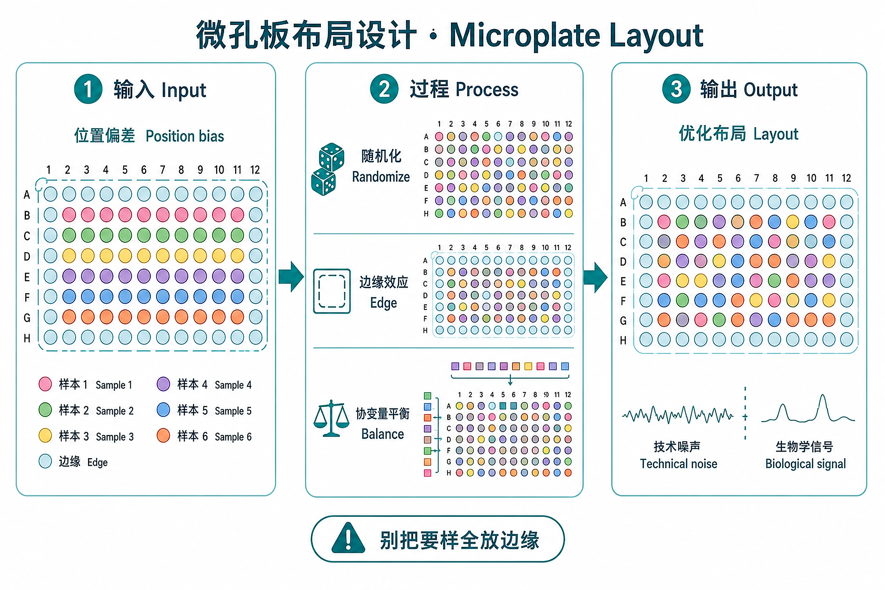
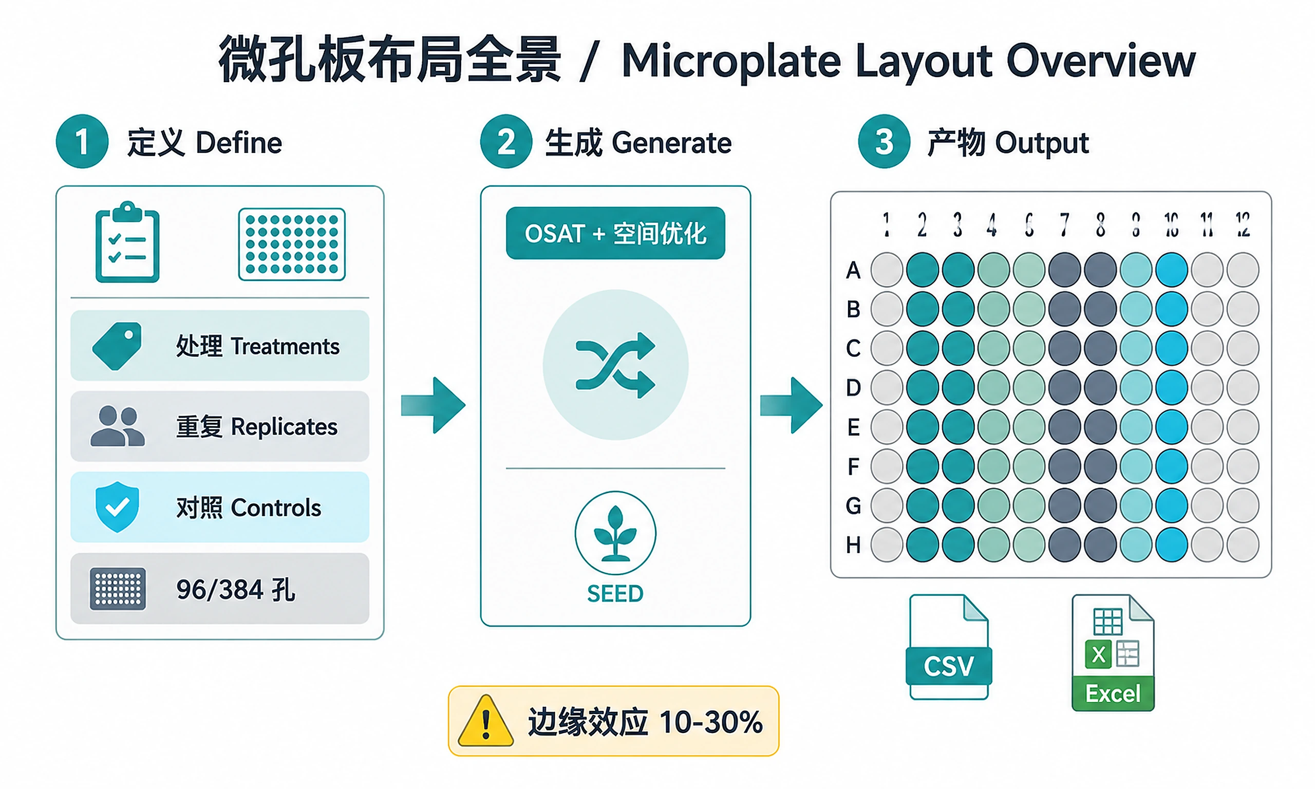
Generate optimized well-plate layouts that minimize positional bias, handle edge effects, balance covariates, and distribute controls across the plate. Exports lab-ready plate maps (images, CSV, Excel) and educates users on common design pitfalls.
When to Use This Skill
Use this skill when you need to:
- ✅ Design a plate layout for any 96-well or 384-well experiment
- ✅ Randomize sample placement to prevent positional confounding
- ✅ Handle edge effects by reserving outer wells or placing controls strategically
- ✅ Balance covariates across plate positions (treatment, replicate, batch)
- ✅ Place controls optimally distributed across all plate quadrants
- ✅ Generate plate maps for the lab bench (images, color-coded Excel, CSV)
- ✅ Learn plate design principles — edge effects, pseudoreplication, randomization
Don't use this skill for:
- ❌ Genomics-specific power analysis (RNA-seq depth, ATAC-seq peaks) → Use
experimental-design-statistics - ❌ Batch assignment across experiments → Use
experimental-design-statistics - ❌ Analyzing plate reader data → Use assay-specific analysis skills
Installation
Required Software
| Software | Version | License | Commercial Use | Installation |
|---|---|---|---|---|
| designit | ≥0.5.0 | MIT | ✅ Permitted | install.packages('designit') |
| ggplot2 | ≥3.3.0 | MIT | ✅ Permitted | install.packages('ggplot2') |
| ggprism | ≥1.0.3 | GPL (≥3) | ✅ Permitted | install.packages('ggprism') |
| jsonlite | ≥1.7.0 | MIT | ✅ Permitted | install.packages('jsonlite') |
| pwr | ≥1.3.0 | GPL (≥3) | ✅ Permitted | install.packages('pwr') |
| ggplate | ≥0.1.0 | MIT | ✅ Permitted | install.packages('ggplate') |
Optional (for enhanced output)
| Software | Version | License | Commercial Use | Installation |
|---|---|---|---|---|
| openxlsx | ≥4.2.0 | MIT | ✅ Permitted | install.packages('openxlsx') |
| agricolae | ≥1.3.0 | GPL-2 | ✅ Permitted | install.packages('agricolae') |
| plater | ≥1.0.0 | GPL-2 | ✅ Permitted | install.packages('plater') |
| patchwork | ≥1.1.0 | MIT | ✅ Permitted | install.packages('patchwork') |
Quick install:
install.packages(c("designit", "ggplot2", "ggprism", "jsonlite", "ggplate",
                    "openxlsx", "agricolae", "plater", "patchwork", "pwr"))
Inputs
Required:
- Experiment definition: plate format, treatments, replicates, controls
Optional:
- Sample metadata file (CSV/TSV) with treatment assignments and covariates
batch_design.rdsfromexperimental-design-statisticsfor multi-plate experiments- Reserved well positions, pipetting constraints
Outputs
Visualizations (PNG + SVG):
plate_treatment_map— Color-coded plate layout by treatment groupplate_sample_type_map— Layout showing samples, controls, empty wellsplate_replicate_map— Distribution of replicates across the plateplate_edge_risk— Heatmap of edge effect susceptibilityplate_quality_dashboard— Quality scores and layout summary- Multi-plate: Per-plate images (
plate_treatment_map_plate1, etc.) using ggplate round wells for high quality
Data files:
plate_layout.csv— Tidy format (one row per well with all metadata)plate_layout_grid.csv— Plate-shaped CSV (rows = plate rows, cols = plate columns)plate_layout.xlsx— Color-coded Excel workbook for the lab benchexperiment_parameters.json— All design parameters (human-readable)layout_quality_report.txt— Quality metrics and recommendations
Analysis objects (RDS):
layout_object.rds— Complete layout for downstream use (includes power analysis)- Load with:
layout <- readRDS('layout_object.rds') analysis_report.pdf— Comprehensive PDF report with Introduction, Methods, Results, Conclusions, and embedded figures
⚠️ PDF style rules:
- US Letter page size (8.5 × 11 in) — always set page dimensions explicitly; do not rely on library defaults
- No Unicode superscripts — use
3.36e-06or3.36 × 10^(-6), not Unicode superscript chars (they render as ■ in PDF fonts) - No half-empty pages — group headings with their content; only page-break before major sections (Results, Conclusions)
- Figures ≥80% page width — multi-panel figures must be large enough to read; never embed below 50% width
Power analysis outputs (requires pwr package):
power_curve.png+.svg— Power vs. replicates curve with current design highlighted- Power metrics included in
layout_quality_report.txtandexperiment_parameters.json
Clarification Questions
🚨 ALWAYS ask Question 1 FIRST. Do not ask about treatments, plate format, or experiment parameters before the user has answered Question 1.
1. Input Files (ASK THIS FIRST):
- Do you have a sample metadata file (CSV/TSV) defining your experiment?
- If uploaded: Does it contain treatment/condition columns and sample IDs?
- Expected formats: CSV/TSV with treatment assignments and covariates
- Or use example data for testing?
- Available:
dose_response_96(6-plate, ≥80% technical + biological power),qpcr_96,cell_viability_384,simple_96 - Use
load_example_experiment("dose_response_96")— all parameters pre-defined
- Available:
🚨 IF EXAMPLE DATA SELECTED: All parameters are pre-defined. DO NOT ask questions 2-7. Proceed directly to Step 1 with
load_example_experiment().
Questions 2-7 are ONLY for users providing their own data:
2. Plate Format: 96-well (8×12, most common) or 384-well (16×24)?
3. Experiment Type: Cell-based assay, qPCR, ELISA, drug screening, or other?
4. Treatments and Replicates: How many conditions? Names? Replicates per condition? Unsure → run power analysis (small/medium/large effect).
5. Controls: Positive control? Negative/vehicle? Blanks? (names and well counts)
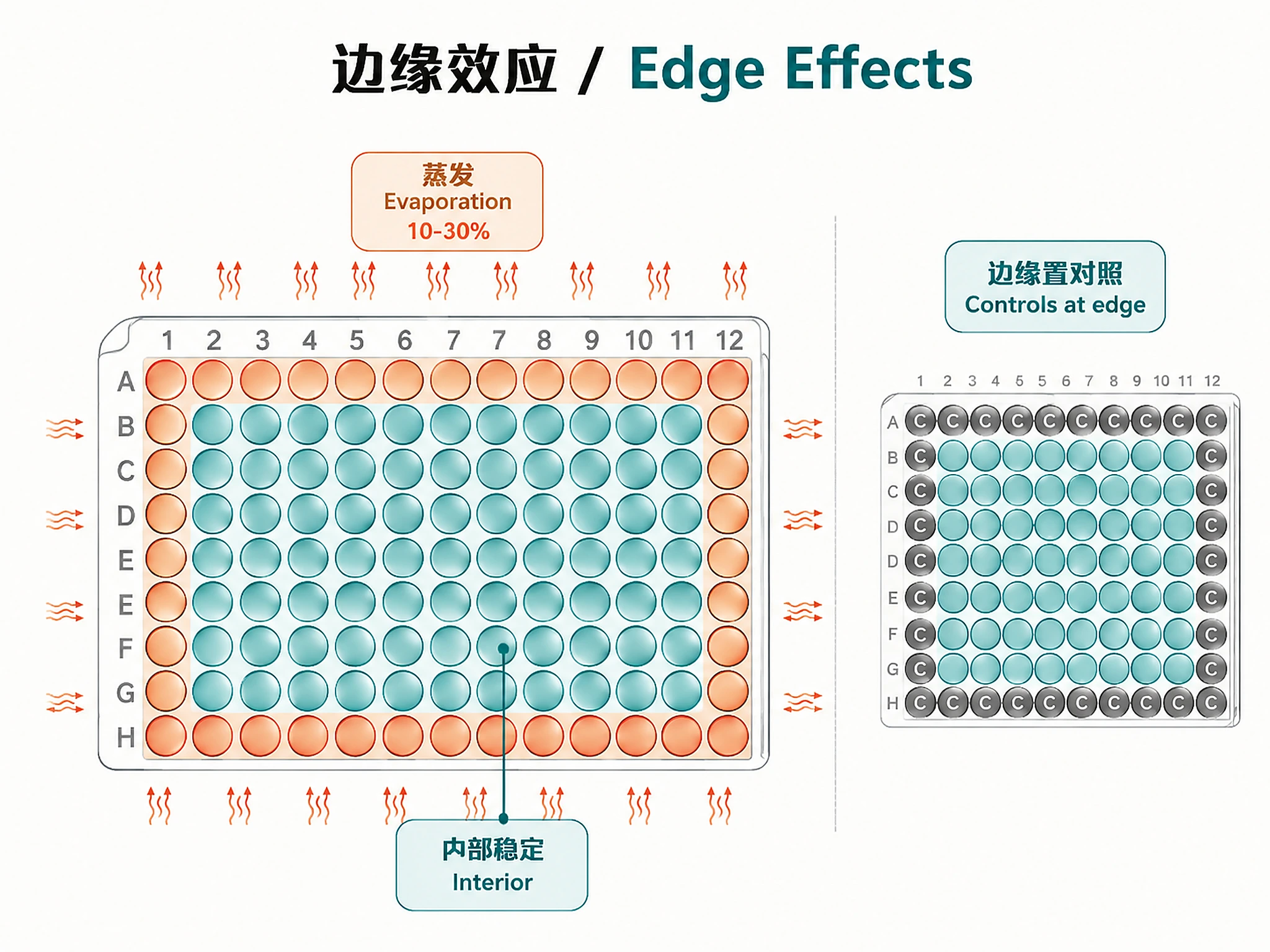
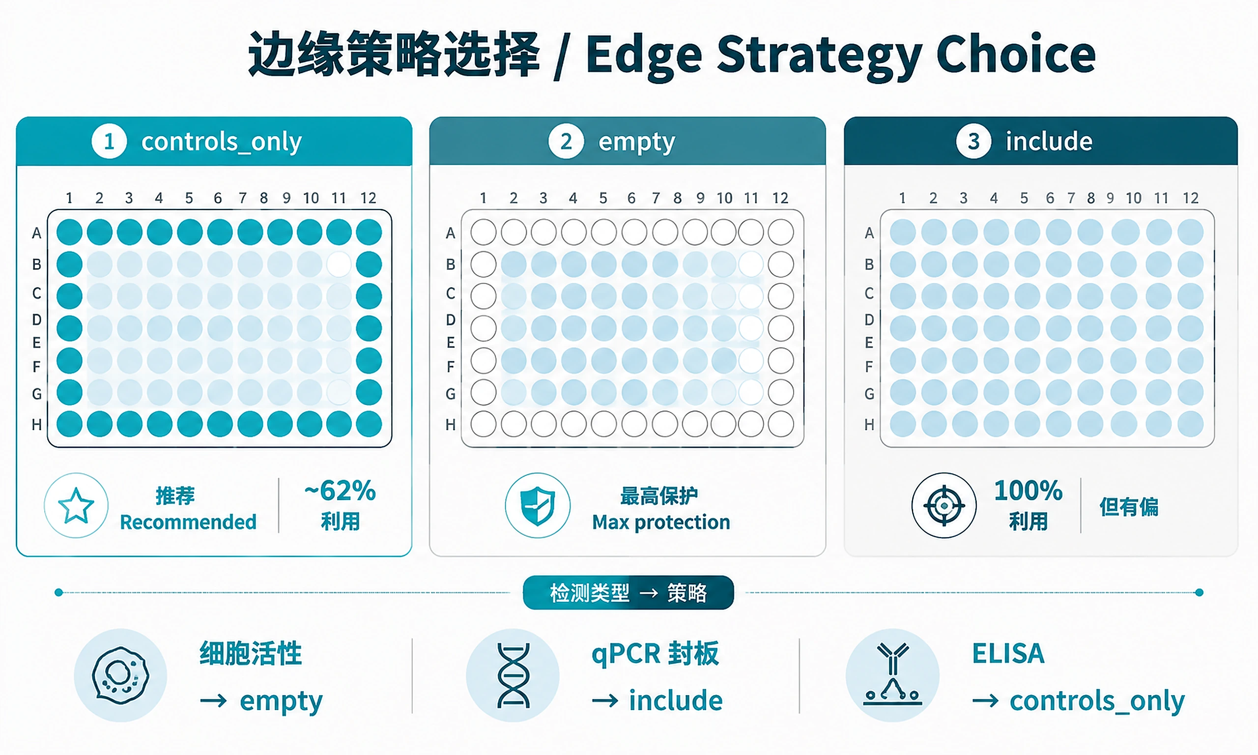
6. Edge Effect Strategy:
"controls_only"(recommended) — Edge wells for controls only; ~62% sample utilization on 96-well but high protection"empty"— Edge wells left empty; same utilization, highest protection"include"— All wells used; 100% utilization but vulnerable to edge effects (10-30% evaporation bias)
7. Additional Parameters (only if user mentions): Multi-plate, covariates, pipetting constraints, reserved wells?
Standard Workflow
🚨 MANDATORY: USE SCRIPTS EXACTLY AS SHOWN - DO NOT WRITE INLINE CODE 🚨
This skill uses low-freedom script execution. You must:
- Source the scripts using the exact commands below
- Wait for verification messages after each step
- NOT write inline code for any step
- NOT modify commands unless explicitly adapting for user-specific data
The plate layout workflow follows 4 steps: Define → Generate → Visualize → Export
Optional: Pre-Design Power Analysis
If the user is unsure about how many replicates to use:
source("scripts/power_analysis.R")
suggestion <- suggest_replicates(
    n_treatments = 3,
    effect_size = "medium",
    plate_format = 96,
    edge_strategy = "controls_only"
)
Use suggestion$required_n as n_replicates in Step 1.
✅ VERIFICATION: You MUST see: "✓ Power-based replicate suggestion completed successfully!"
Step 1 - Define Experiment
source("scripts/load_example_experiment.R")
experiment <- load_example_experiment("dose_response_96")
Or define interactively:
source("scripts/load_example_experiment.R")
experiment <- define_experiment(
    plate_format = 96,
    treatments = c("Drug", "Vehicle"),
    n_replicates = 5,
    controls = list(positive = "Staurosporine", negative = "DMSO", blank = "Media"),
    n_controls = list(positive = 4, negative = 4, blank = 4),
    edge_strategy = "controls_only",
    n_plates = 6
)
DO NOT write inline experiment definition code. Use load_example_experiment() or define_experiment().
✅ VERIFICATION: You MUST see: "✓ Experiment defined successfully!"
Available examples: dose_response_96, qpcr_96, cell_viability_384, simple_96
Step 2 - Generate Layout
source("scripts/generate_layout.R")
layout <- generate_plate_layout(
    experiment,
    method = "osat_spatial",
    seed = 42
)
DO NOT write inline randomization or assignment code. Use the script.
Methods:
"osat_spatial"(default) — OSAT + spatial optimization via designit"block_random"— Block randomization with spatial constraints"latin_square"— Latin square mapped to plate coordinates"manual_template"— Start from a template, modify manually
⚠️ CRITICAL - DO NOT:
- ❌ Write inline sample assignment code → STOP: Use
generate_plate_layout() - ❌ Manually place samples in wells → STOP: Use the optimization methods
- ❌ Skip randomization → confounds treatment with plate position
✅ VERIFICATION: You MUST see: "✓ Layout generated successfully!"
Quality check: Score should be ≥80%. If lower, try: different seed, more iterations (max_iter = 2000), or different method.
Then complete ALL sub-steps 2a–2e in order:
Step 2a — Assess statistical power (MANDATORY):
source("scripts/power_analysis.R")
layout <- assess_layout_power(layout, effect_size = "medium")
Effect size options: "small" (subtle differences), "medium" (typical/moderate), "large" (obvious). Resolves to Cohen's d (t-test) or Cohen's f (ANOVA) automatically.
Choose effect size by assay type:
- Dose-response / cell viability: For full dose-response curves (concentrations spanning IC50), use
"large"(d=0.8) or a numeric value like2.0for strong cytotoxic effects (>50% viability change). For sub-IC50 screening or assays targeting subtle viability shifts, use"medium"(d=0.5) — not all dose points produce large effects. The demo uses d=2.0 to demonstrate adequate biological power across 6 independent preparations. - Gene expression / proteomics: Use
"medium"— moderate fold-changes between conditions - Subtle phenotypes / biomarkers: Use
"small"— detecting weak effects requires more replicates
DO NOT skip power assessment. ALWAYS run assess_layout_power() after generating the layout.
✅ VERIFICATION: You MUST see: "✓ Power assessment completed successfully!"
⚠️ MANDATORY: If power < 0.80, you MUST stop and present the user with options:
- Add plates — Increase
n_platesin Step 1 to spread replicates across multiple plates (usesuggest_replicates()to find the right total n, then divide across plates) - Increase replicates per plate — If wells are available, increase
n_replicates - Accept underpowered design — Proceed only with explicit user acknowledgment that the design may miss real effects
- Target larger effect size — Re-run
assess_layout_power(layout, effect_size = "large")to check if adequate for large effects only
DO NOT silently proceed with an underpowered design. DO NOT reassure the user that low power is "typical" or "expected."
⚠️ MANDATORY — Biological Replication Plan:
assess_layout_power() reports a Biological Replication Plan showing how many independent experiments are needed for adequate biological power. You MUST:
- Present the biological replication plan prominently — not as a footnote
- State the required number of independent preparations for 80% biological power
- Show power at 3 and 5 independent preparations so the user understands the tradeoff
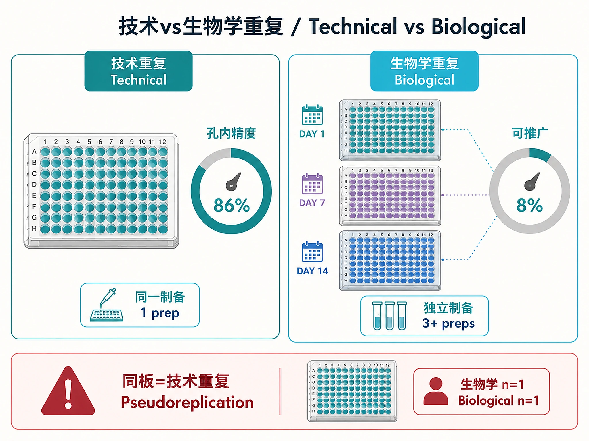
- Explain: Technical power validates the plate layout; biological power requires independent experimental days/cell preparations. Wells within a plate are technical replicates — they cannot substitute for biological replication.
DO NOT present technical power alone as evidence the design is adequate. DO NOT minimize the biological power limitation. A well-designed plate with 86% technical power but 8% biological power means: the plate layout is efficient, but you need more independent experiments for generalizable conclusions.
⚠️ DO NOT claim power for effect sizes that were NOT tested. If you only ran effect_size = "medium", you may NOT state the design is "well-powered for large effects" without running assess_layout_power(layout, effect_size = "large") to verify.
⚠️ MANDATORY — Effect Size Sensitivity Table:
assess_layout_power() automatically computes a sensitivity table showing power at small, medium, large, and your chosen effect size. You MUST:
- Present the sensitivity table to the user — do NOT only report the chosen effect size's power
- Discuss whether the chosen effect size is realistic for the user's assay. For example, d=2.0 assumes >50% viability change; many drug treatments produce smaller effects
- Flag when medium-effect biological power is low — the script warns automatically, but you should explain what this means practically
Step 2b — Power curve plot:
plot_power_curve(
    n_treatments = length(layout$experiment$treatments),
    effect_size = "medium",
    current_n = layout$power_analysis$min_n_per_group,
    output_dir = "layout_results"
)
✅ VERIFICATION: You MUST see: "✓ Power curve generated successfully!"
CRITICAL — Two Kinds of Power:
- Technical power (well-level): Validates the plate layout — enough wells to measure precisely within each experiment. This is what the script checks against 80%.
- Biological power (experiment-level): Determines ability to generalize conclusions. Requires independent experiments (different days, cell passages, preparations). Almost always requires 3+ independent preparations.
A design can have 86% technical power and 8% biological power simultaneously. Both numbers are correct but answer different questions. The agent MUST present the full Biological Replication Plan from
assess_layout_power()showing power at 3, 5, and the required number of independent preparations.
Step 2c — Comprehensive confounding check (MANDATORY):
confounding <- check_all_confounding(layout)
✅ VERIFICATION: You MUST see: "✓ Comprehensive confounding check completed successfully!"
This tests quadrant, row, column, edge, and plate-level (if multi-plate) confounding.
If any check reports FAILED (p ≤ 0.05), re-run generate_plate_layout() with a different seed or method.
⚠️ IF CONFOUNDING DETECTED AND YOU CHANGE THE SEED: You MUST re-run ALL of Steps 2a-2c with the new layout:
- Re-run
assess_layout_power()— power analysis from the old seed is invalid- Re-run
plot_power_curve()— the old power curve belongs to the old layout- Re-run
check_all_confounding()— verify the new seed passes Do NOT reuse power curves, power analysis results, or visualizations from a previous layout/seed.
IF confounding is detected (seed fails): Explain to the user why this matters — the initial seed produced a layout with positional confounding (treatment correlated with plate position). This demonstrates that not all random layouts are confounding-free, which is why automated confounding checks are essential. The layout may look acceptable visually but harbor hidden statistical biases.
Step 2d — Explain design principles to user (MANDATORY):
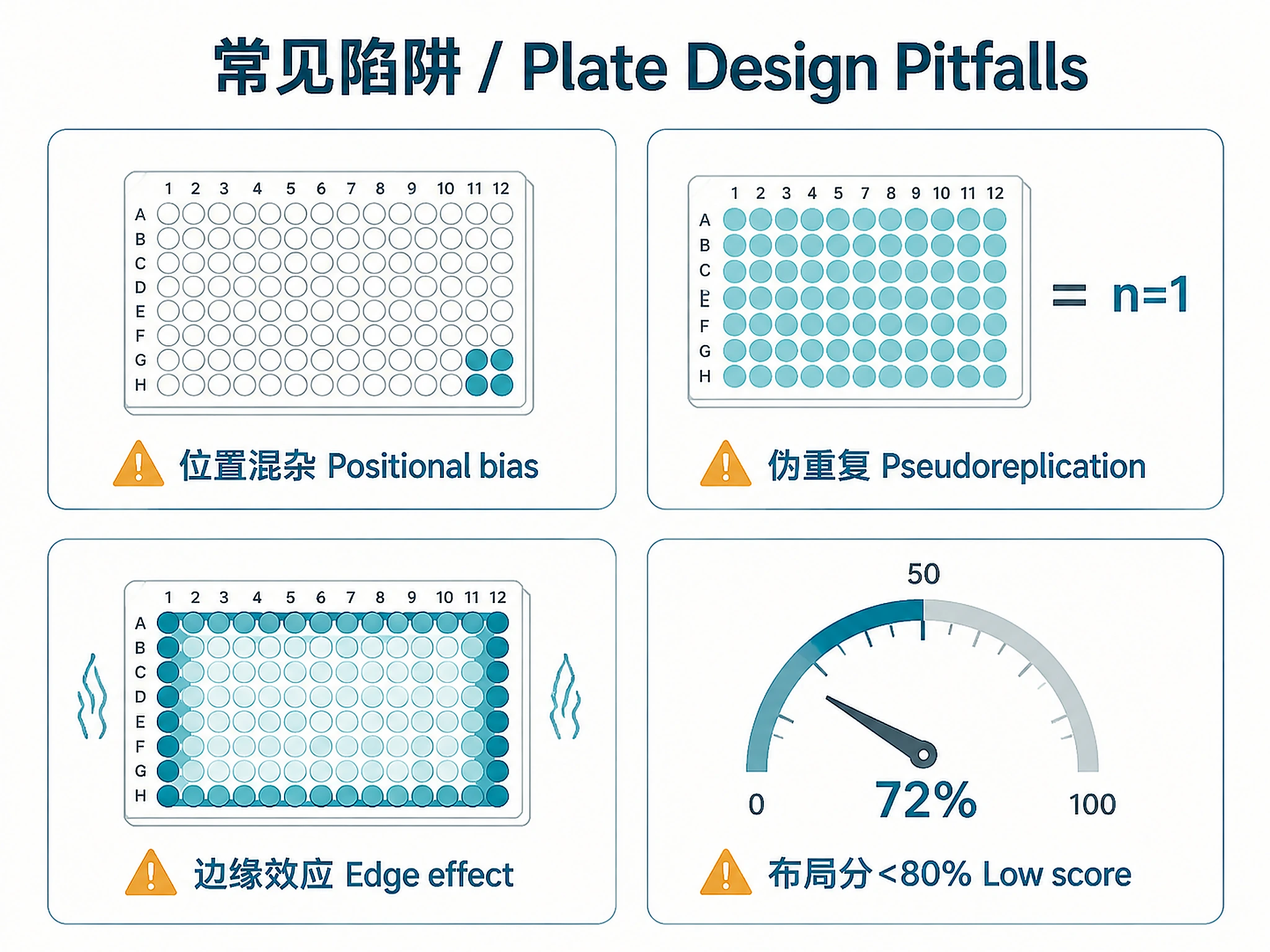
🚨 You MUST Read("references/design_principles.md") and quote specific numbers from it. Do NOT explain from memory or from this SKILL.md. 🚨
Read references/design_principles.md and explain to the user:
- Quote the 10-30% evaporation bias figure from Section 1 (Edge Effects)
- Present the full 3-row edge well utilization comparison table from Section 1 (the one with Strategy / Protection / Usable Wells / When to Use columns) — do NOT summarize in prose; show the complete table so users can compare strategies at a glance
- Quote the pseudoreplication definition from Section 3 — wells on the same plate are technical replicates. With a single plate, biological n = 1 per treatment regardless of well count. Multi-plate experiments with independent preparations provide true biological replication.
Step 2e — Discuss edge strategy tradeoff:
🚨 Read references/design_principles.md Section 1 and present the edge strategy table from the reference document. Do NOT reproduce from memory. 🚨
Present the full edge strategy tradeoff table for the user's specific assay type (do not summarize — show the complete table):
| Assay Type | Recommended Strategy | Rationale |
|---|---|---|
| Cell viability (open plate, >24h) | empty or controls_only |
10-30% evaporation bias in outer wells |
| qPCR (sealed plates) | include |
Sealed plates minimize evaporation; recovers ~38% more wells |
| ELISA (short incubation) | controls_only |
Controls in edges detect plate-level drift |
| Drug screen (384-well) | empty |
384-well plates have more severe edge effects |
| Cell-based (sealed, <6h) | include or controls_only |
Minimal edge bias with sealed short incubations |
Why
controls_onlyoverempty? Both strategies reserve edge wells and yield the same number of interior wells for samples. The difference:controls_onlyplaces controls in edge wells, providing quantitative data about edge-specific behavior (evaporation, signal drift) that can inform normalization. Withempty, those wells generate no data. Useemptyonly when reagent cost prohibits edge controls or when edge contamination risk is severe.
For details, read references/design_principles.md Section 1 (Edge Effects).
Step 3 - Generate Visualizations
source("scripts/visualize_plate.R")
visualize_all_plates(layout, output_dir = "layout_results")
DO NOT write inline plotting code (ggsave, ggplot, geom_tile, geom_point, etc.). Just use the script.
DO NOT create your own plate map plots. The script uses ggplate round-well style + ggprism theme.
The script generates 5 publication-quality plots using ggplate (round wells) with ggprism theme, plus PNG + SVG export with graceful fallback.
✅ VERIFICATION: You MUST see: "✓ All plots generated successfully!"
Step 4 - Export Results
source("scripts/export_layout.R")
export_all(layout, output_dir = "layout_results")
DO NOT write custom export code. Use export_all().
✅ VERIFICATION: You MUST see: "=== Export Complete ==="
DEMO DATA DISCLAIMER (MANDATORY): If example data was used, you MUST include this notice prominently in your final summary: "This layout was generated using the built-in [example_name] demo dataset for demonstration purposes only. To design a layout for your actual experiment, re-run from Step 1 with
define_experiment()using your own treatments, replicates, and controls."
⚠️ CRITICAL - DO NOT:
- ❌ Skip power assessment → STOP: ALWAYS run
assess_layout_power()andplot_power_curve()in Step 2 - ❌ Write inline experiment definition code → STOP: Use
define_experiment()orload_example_experiment() - ❌ Write inline sample assignment or randomization code → STOP: Use
generate_plate_layout() - ❌ Write inline plotting code (ggsave, ggplot, geom_tile, geom_point, plate maps, etc.) → STOP: Use
visualize_all_plates()— it uses ggplate round-well style + ggprism theme - ❌ Write custom export code → STOP: Use
export_all() - ❌ Try to install svglite → script handles SVG fallback automatically
- ❌ Use absolute paths or setwd() → use relative paths only
- ❌ Claim power for untested effect sizes → STOP: If you only tested "medium", you CANNOT claim "well-powered for large effects" without running
assess_layout_power(layout, effect_size = "large") - ❌ Proceed silently when underpowered (power < 0.80) → STOP: You MUST present options to the user (add plates, increase replicates, accept, or test different effect size)
- ❌ Skip confounding check → STOP: ALWAYS run
check_layout_confounding(layout)in Step 2c
✅ VERIFICATION - You MUST see ALL of these:
- After Step 1:
"✓ Experiment defined successfully!" - After Step 2:
"✓ Layout generated successfully!"AND"✓ Power assessment completed successfully!"AND"✓ Power curve generated successfully!"AND"✓ Confounding check completed successfully!" - After Step 3:
"✓ All plots generated successfully!" - After Step 4:
"=== Export Complete ==="
❌ IF YOU DON'T SEE THESE MESSAGES: You wrote inline code. Stop and use source() with the scripts above.
⚠️ IF SCRIPTS FAIL - Script Failure Hierarchy:
- Fix and Retry (90%) - Install missing package, re-run script
- Modify Script (5%) - Edit the script file itself, document changes
- Use as Reference (4%) - Read script, adapt approach, cite source
- Write from Scratch (1%) - Only if genuinely impossible, explain why
NEVER skip directly to writing inline code without trying the script first.
Common Issues
| Issue | Cause | Solution |
|---|---|---|
| "Not enough available wells" | Too many samples for plate format | Reduce replicates, add plates (n_plates), or switch to 384-well |
| Low quality score (<80%) | Poor spatial distribution | Increase max_iter, try different seed, or use osat_spatial method |
| Controls not in all quadrants | Not enough control wells | Increase n_controls (minimum 4 per type for 96-well) |
| designit not found | Package not installed | install.packages('designit') |
| ggplate not found | Required package missing | install.packages('ggplate') — required for plate visualizations |
| SVG export error | Missing svglite dependency | Normal — scripts fall back to base R svg() or skip SVG. PNG always works. |
| Excel export skipped | openxlsx not installed | install.packages('openxlsx') — CSV exports always available |
| Power < 0.80 | Insufficient replicates for effect size | Add plates (n_plates), increase n_replicates, or use suggest_replicates() to find optimal n |
| pwr not installed | Required power analysis package missing | install.packages('pwr') — needed for mandatory power assessment |
Suggested Next Steps
After generating your plate layout:
- Print the plate map — Use
plate_treatment_map.pngor the Excel file for the bench - Review the quality report — Check
layout_quality_report.txtfor recommendations - Run the experiment — Follow the plate map for sample placement
- After data collection — Use
plate_layout.csvto merge layout with reader data - Consider b-score normalization — If edge effects detected in data, use
platetools::b_score()
Related Skills
Upstream:
- experimental-design-statistics — Power analysis, sample size, batch assignment across plates
- Its
batch_design.rdscan inform multi-plate sample assignment
Downstream:
- de-results-to-plots — Visualize experimental results
- bulk-rnaseq-counts-to-de-deseq2 — If the plate experiment feeds into RNA-seq
References
Scripts: See scripts/ for all functions:
- load_example_experiment.R — Example experiments +
define_experiment() - generate_layout.R — Layout generation engine
- visualize_plate.R — Plate visualizations
- export_layout.R — Multi-format export
- power_analysis.R — Power analysis, replicate suggestion, confounding check
Reference docs:
- design_principles.md — Edge effects, pseudoreplication, randomization, controls
- plate_formats.md — 96-well and 384-well specifications
- common_assay_layouts.md — qPCR, ELISA, dose-response templates
- advanced_designs.md — Latin square, multi-plate, OSAT details
Key papers:
- Wollmann et al. (2023) SLAS Discovery — AI-optimized microplate layouts (PLAID)
- Borbouse et al. (2021) Bioinformatics — Well Plate Maker randomization
- Lazic SE (2010) BMC Neuroscience — Pseudoreplication in biological experiments
- Murphy TJ — Sampling and Experimental Units
Code preview
scripts/export_layout.R
# =============================================================================
# Microplate Layout Design - Export Results
# =============================================================================
# Exports plate layouts in multiple formats for lab use and downstream analysis.
# =============================================================================

suppressPackageStartupMessages({
    library(jsonlite)
})

# --- Main export function ---
export_all <- function(layout, experiment = NULL, output_dir = "layout_results") {
    if (!inherits(layout, "plate_layout")) {
        stop("Input must be a 'plate_layout' object from generate_plate_layout()")
    }

    if (is.null(experiment)) experiment <- layout$experiment
    dir.create(output_dir, showWarnings = FALSE, recursive = TRUE)

    cat("\n=== Exporting Plate Layout ===\n")
    cat("Output directory:", output_dir, "\n\n")

    plate_data <- layout$plate_data

    # 1. Tidy CSV (one row per well)
    cat("1. Tidy CSV (plate_layout.csv)...\n")
    tidy_df <- plate_data[, c("plate", "well", "row_label", "col_label",
                               "row", "col", "is_edge", "well_role",
                               "sample_id", "treatment", "replicate", "sample_type")]
    write.csv(tidy_df, file.path(output_dir, "plate_layout.csv"), row.names = FALSE)
    cat("   Saved:", file.path(output_dir, "plate_layout.csv"), "\n")

    # 2. Plate-shaped grid CSV (one per plate)
    cat("2. Grid CSV (plate_layout_grid.csv)...\n")
    for (p in 1:experiment$n_plates) {
        plate_subset <- plate_data[plate_data$plate == p, ]
        dims <- experiment$plate_dims

        # Create a matrix with well contents
        grid <- matrix("", nrow = dims$rows, ncol = dims$cols)
        rownames(grid) <- dims$row_labels
        colnames(grid) <- dims$col_labels

        for (i in seq_len(nrow(plate_subset))) {
            r <- plate_subset$row[i]
            c <- plate_subset$col[i]
            content <- plate_subset$sample_id[i]
            if (is.na(content)) {
                if (plate_subset$well_role[i] == "empty") {
                    content <- "[EMPTY]"
                } else {
                    content <- ""
                }
            }
            grid[r, c] <- content
        }

        suffix <- if (experiment$n_plates > 1) paste0("_plate", p) else ""
        grid_path <- file.path(output_dir, paste0("plate_layout_grid", suffix, ".csv"))
        write.csv(grid, grid_path)
        cat("   Saved:", grid_path, "\n")
    }

    # 3. Excel with color-coded cells (if openxlsx available)
    cat("3. Excel workbook (plate_layout.xlsx)...\n")
    if (requireNamespace("openxlsx", quietly = TRUE)) {
        tryCatch({
            .export_excel(layout, experiment, output_dir)
        }, error = function(e) {
            cat("   Excel export failed:", conditionMessage(e), "\n")
            cat("   (CSV exports are available as alternative)\n")
        })
    } else {
        cat("   (openxlsx not available - skipping Excel export)\n")
    }

    # 4. Layout object (RDS)
    cat("4. Layout object (layout_object.rds)...\n")
    saveRDS(layout, file.path(output_dir, "layout_object.rds"))
    cat("   Saved:", file.path(output_dir, "layout_object.rds"), "\n")
scripts/generate_layout.R
# =============================================================================
# Microplate Layout Design - Core Layout Generation Engine
# =============================================================================
# Generates optimized plate layouts using designit (OSAT + spatial scoring),
# agricolae (Latin square), or block randomization.
# =============================================================================

suppressPackageStartupMessages({
    library(designit)
    library(ggplot2)
})

# --- Main layout generation function ---
generate_plate_layout <- function(experiment,
                                   method = "osat_spatial",
                                   balance_vars = NULL,
                                   seed = 42,
                                   max_iter = 1000,
                                   quiet = FALSE) {

    if (!inherits(experiment, "plate_experiment")) {
        stop("Input must be a 'plate_experiment' object from define_experiment()")
    }

    set.seed(seed)
    if (!quiet) cat("\n=== Generating Plate Layout ===\n")
    if (!quiet) cat("Method:", method, "\n")
    if (!quiet) cat("Seed:", seed, "\n\n")

    # Build the sample table
    samples <- .build_sample_table(experiment)

    # Build the plate grid
    plate_grid <- .build_plate_grid(experiment)

    # Mark edge wells, reserved wells
    plate_grid <- .mark_special_wells(plate_grid, experiment)

    # Generate layout based on method
    layout <- switch(method,
        "osat_spatial" = .layout_osat_spatial(plate_grid, samples, experiment,
                                              balance_vars, max_iter, quiet),
        "block_random" = .layout_block_random(plate_grid, samples, experiment,
                                              balance_vars, seed, quiet),
        "latin_square" = .layout_latin_square(plate_grid, samples, experiment, seed, quiet),
        "manual_template" = .layout_manual_template(plate_grid, samples, experiment, quiet),
        stop("Unknown method: ", method,
             ". Use: osat_spatial, block_random, latin_square, manual_template")
    )

    # Place controls
    layout <- .place_controls(layout, experiment, seed, quiet)

    # Score quality
    quality <- .score_layout_quality(layout, experiment)
    layout$quality <- quality

    # Attach experiment metadata
    layout$experiment <- experiment
    layout$method <- method
    layout$seed <- seed
    class(layout) <- "plate_layout"

    if (!quiet) {
        cat("\n✓ Layout generated successfully!\n")
        cat("  Method:", method, "\n")
        cat("  Wells assigned:", sum(!is.na(layout$plate_data$sample_id)), "of",
            nrow(layout$plate_data), "\n")
        cat("  Quality score:", round(quality$overall_score, 2), "/ 1.00\n")
        cat("  Spatial balance:", round(quality$spatial_score, 2), "/ 1.00\n")
        cat("  Control distribution:", round(quality$control_score, 2), "/ 1.00\n")
    }

    return(layout)
}

# --- Build sample table from experiment ---
.build_sample_table <- function(experiment) {
    samples <- data.frame(
        sample_id = character(0),
scripts/load_example_experiment.R
# =============================================================================
# Microplate Layout Design - Example Experiment Definitions
# =============================================================================
# Provides pre-built experiment definitions for testing and demonstration.
# Users can also define experiments interactively with define_experiment().
# =============================================================================

# --- Package check ---
.check_packages <- function() {
    options(repos = c(CRAN = "https://cloud.r-project.org"))
    required <- c("designit", "ggplot2", "jsonlite", "pwr", "ggplate")
    missing <- required[!sapply(required, requireNamespace, quietly = TRUE)]
    if (length(missing) > 0) {
        cat("Installing required packages:", paste(missing, collapse = ", "), "\n")
        install.packages(missing)
    }
    # Optional packages: check availability but do NOT auto-install.
    # Downstream scripts (visualize_plate.R, export_layout.R) handle these
    # gracefully with requireNamespace() checks at point of use.
    optional <- c("openxlsx", "agricolae", "plater", "patchwork")
    available_opt <- sapply(optional, requireNamespace, quietly = TRUE)
    if (!all(available_opt)) {
        missing_opt <- optional[!available_opt]
        cat("  Optional packages not installed:", paste(missing_opt, collapse = ", "), "\n")
        cat("  Install with: install.packages(c('", paste(missing_opt, collapse = "', '"), "'))\n")
        cat("  Core functionality works without them.\n")
    }
}

# --- Plate format definitions ---
.plate_formats <- list(
    "96"  = list(rows = 8,  cols = 12, row_labels = LETTERS[1:8],  col_labels = 1:12),
    "384" = list(rows = 16, cols = 24, row_labels = LETTERS[1:16], col_labels = 1:24)
)

# --- Define experiment interactively ---
define_experiment <- function(plate_format = 96,
                              treatments = c("Treatment_A", "Treatment_B", "Vehicle"),
                              n_replicates = 3,
                              controls = list(positive = NULL, negative = NULL, blank = NULL),
                              n_controls = list(positive = 4, negative = 4, blank = 4),
                              edge_strategy = "controls_only",
                              n_plates = 1,
                              covariates = NULL,
                              reserved_wells = NULL,
                              experiment_name = "Experiment",
                              assay_type = "general") {

    plate_fmt <- .plate_formats[[as.character(plate_format)]]
    if (is.null(plate_fmt)) {
        stop("Unsupported plate format: ", plate_format,
             ". Supported: ", paste(names(.plate_formats), collapse = ", "))
    }

    total_wells <- plate_fmt$rows * plate_fmt$cols * n_plates

    # Calculate edge wells
    edge_wells <- .get_edge_wells(plate_fmt)

    # Calculate available wells based on edge strategy
    if (edge_strategy == "empty") {
        interior_wells <- total_wells - length(edge_wells) * n_plates
        usable_for_samples <- interior_wells
    } else if (edge_strategy == "controls_only") {
        interior_wells <- total_wells - length(edge_wells) * n_plates
        usable_for_samples <- interior_wells
    } else {
        usable_for_samples <- total_wells
    }

    # Calculate total controls needed
    total_controls <- sum(unlist(n_controls[!sapply(controls, is.null)]))

    # Calculate sample wells needed
    n_sample_wells <- length(treatments) * n_replicates * n_plates
    wells_needed <- n_sample_wells + total_controls * n_plates

    # Reserved wells
    n_reserved <- if (!is.null(reserved_wells)) length(reserved_wells) * n_plates else 0
Companion files
| Type | Path | Bytes |
|---|---|---|
| Markdown | references/advanced_designs.md | 4,415 |
| Markdown | references/common_assay_layouts.md | 4,760 |
| Markdown | references/design_principles.md | 9,559 |
| Markdown | references/plate_formats.md | 2,528 |
| R | scripts/export_layout.R | 17,083 |
| R | scripts/generate_layout.R | 21,948 |
| R | scripts/load_example_experiment.R | 8,779 |
| R | scripts/power_analysis.R | 28,112 |
| R | scripts/visualize_plate.R | 16,216 |
| Markdown | SKILL.md | 24,587 |
| JSON | skill.meta.json | 1,822 |