Clinical Survival Analysis
Kaplan-Meier, Cox regression, risk stratification.
Overview
Problem. Do survival times differ; what factors drive risk?
Learning goals
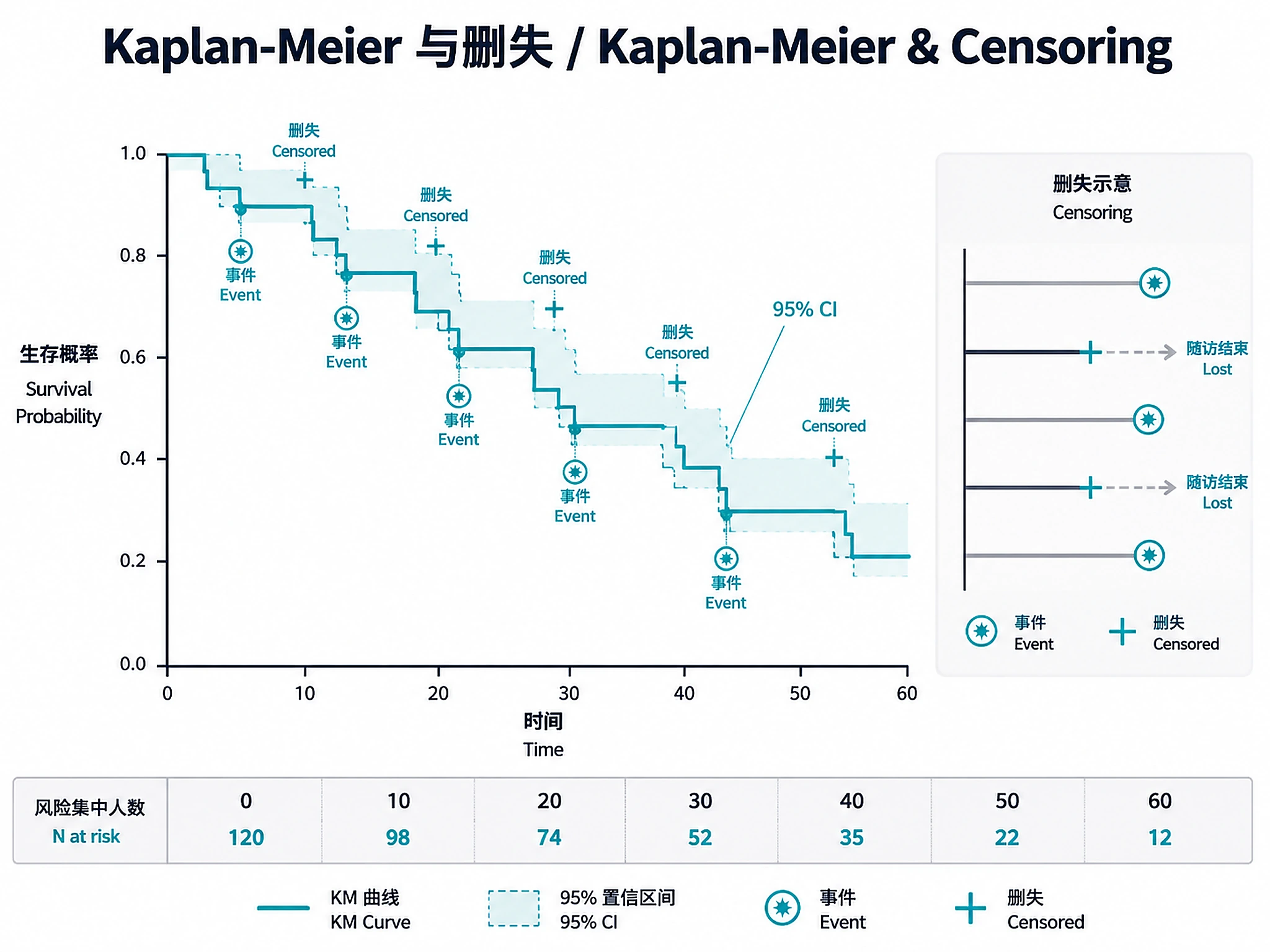
- Censoring is central — keep that information
- Test the proportional-hazards assumption
Figures
Tutorial
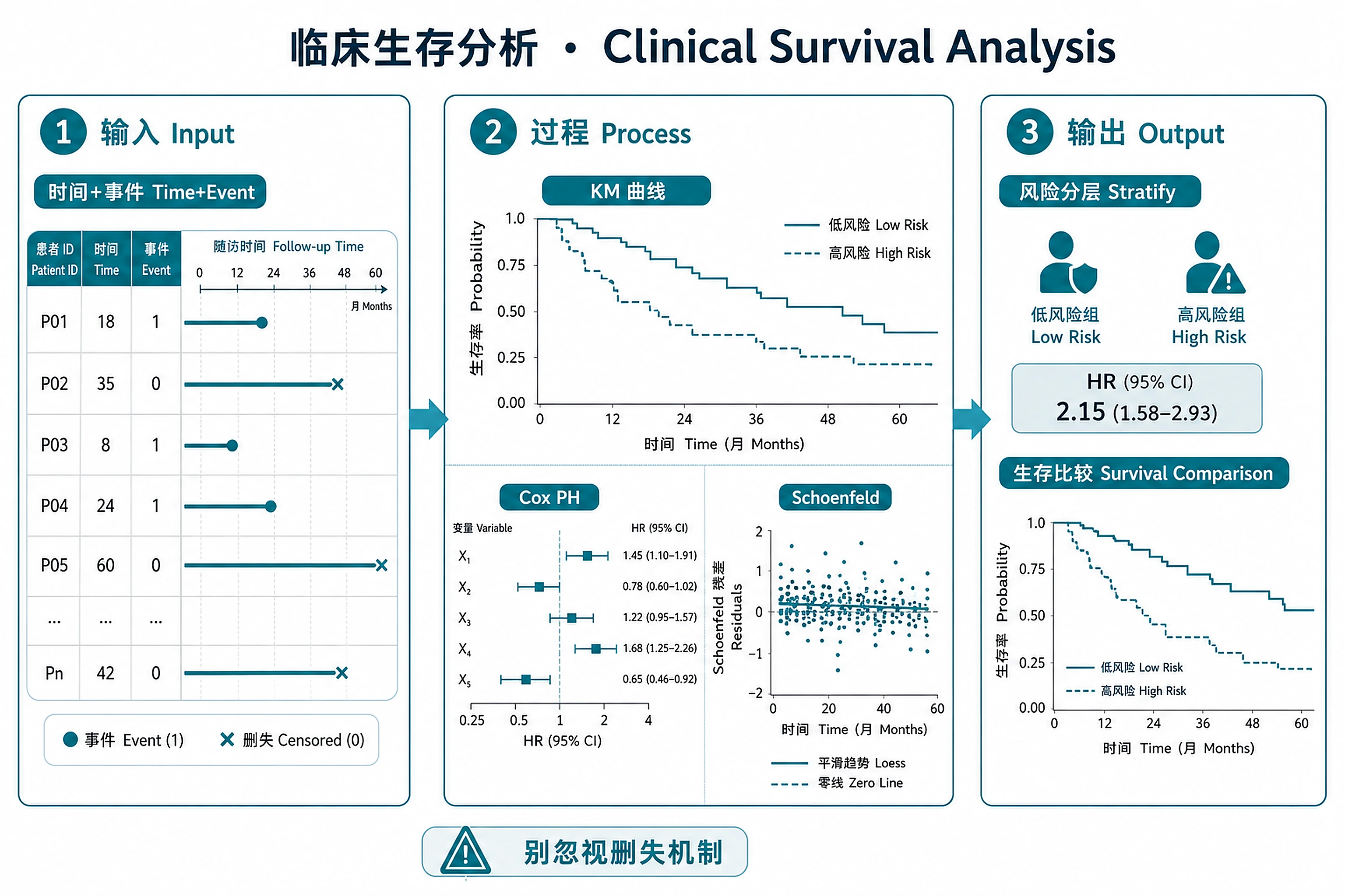
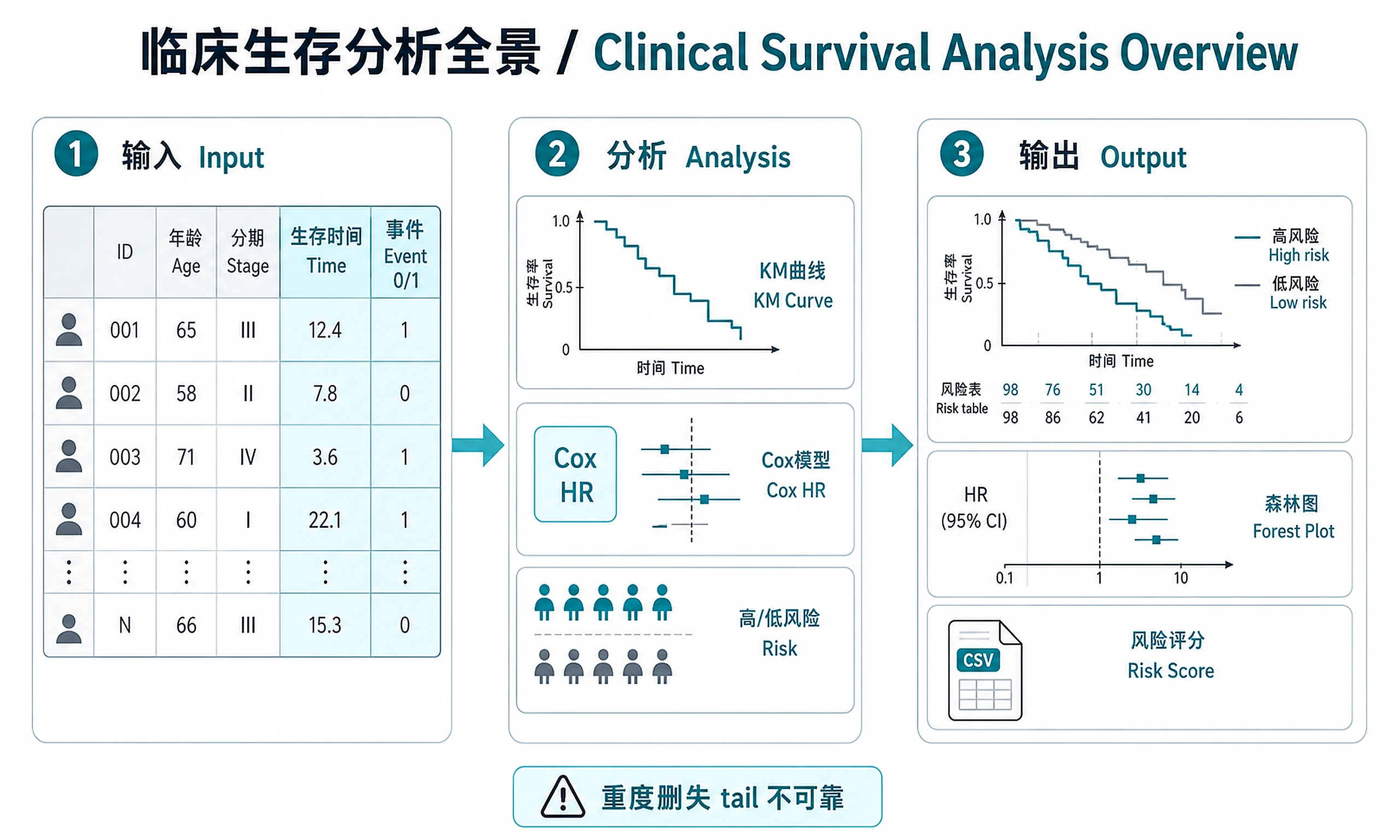
Kaplan-Meier survival estimation, Cox proportional hazards regression, and risk stratification for clinical and real-world evidence (RWE) datasets.
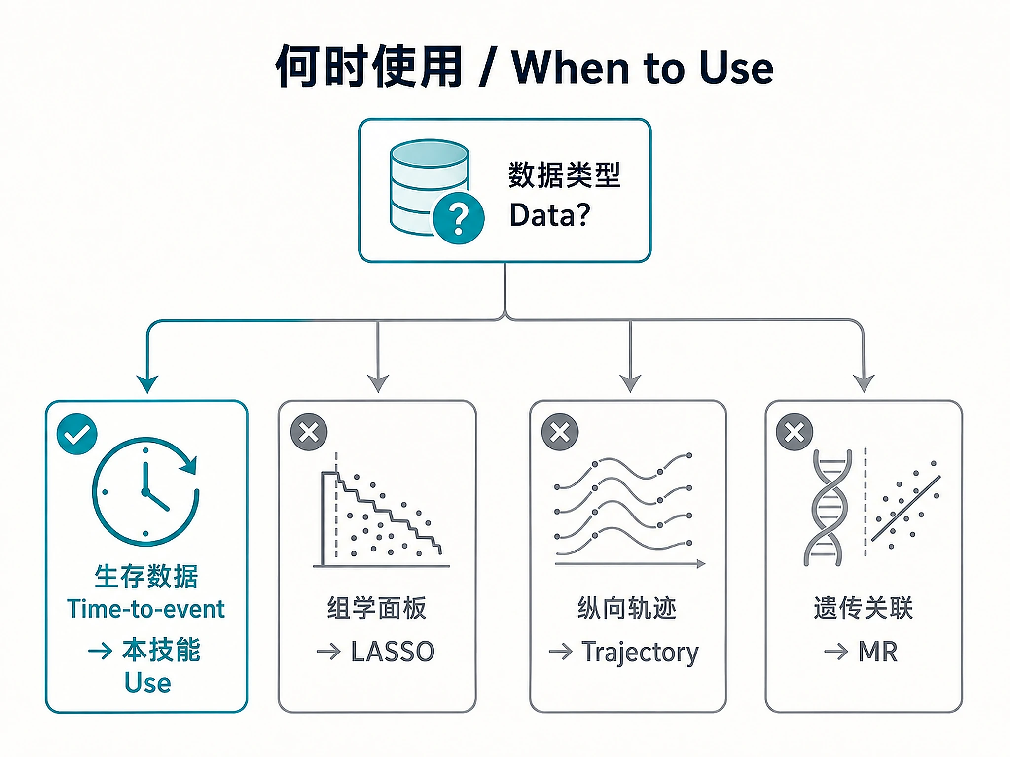
When to Use This Skill
Use this skill when you need to:
- Estimate survival curves (Kaplan-Meier) with confidence intervals and risk tables
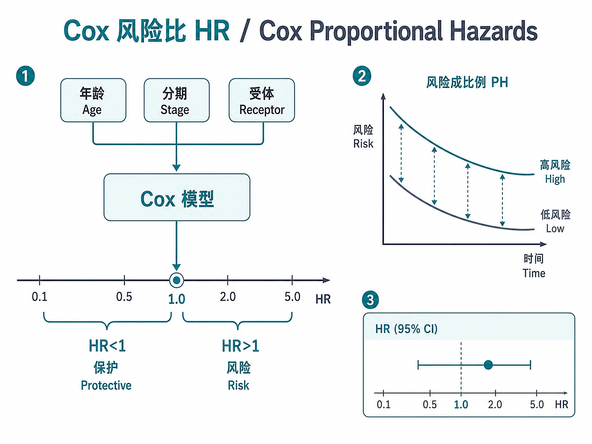
- Identify prognostic factors via Cox proportional hazards regression
- Stratify patients by risk using Cox model linear predictor
- Test proportional hazards assumption with Schoenfeld residuals
- Compare survival between groups (molecular subtypes, treatment arms, biomarker levels)
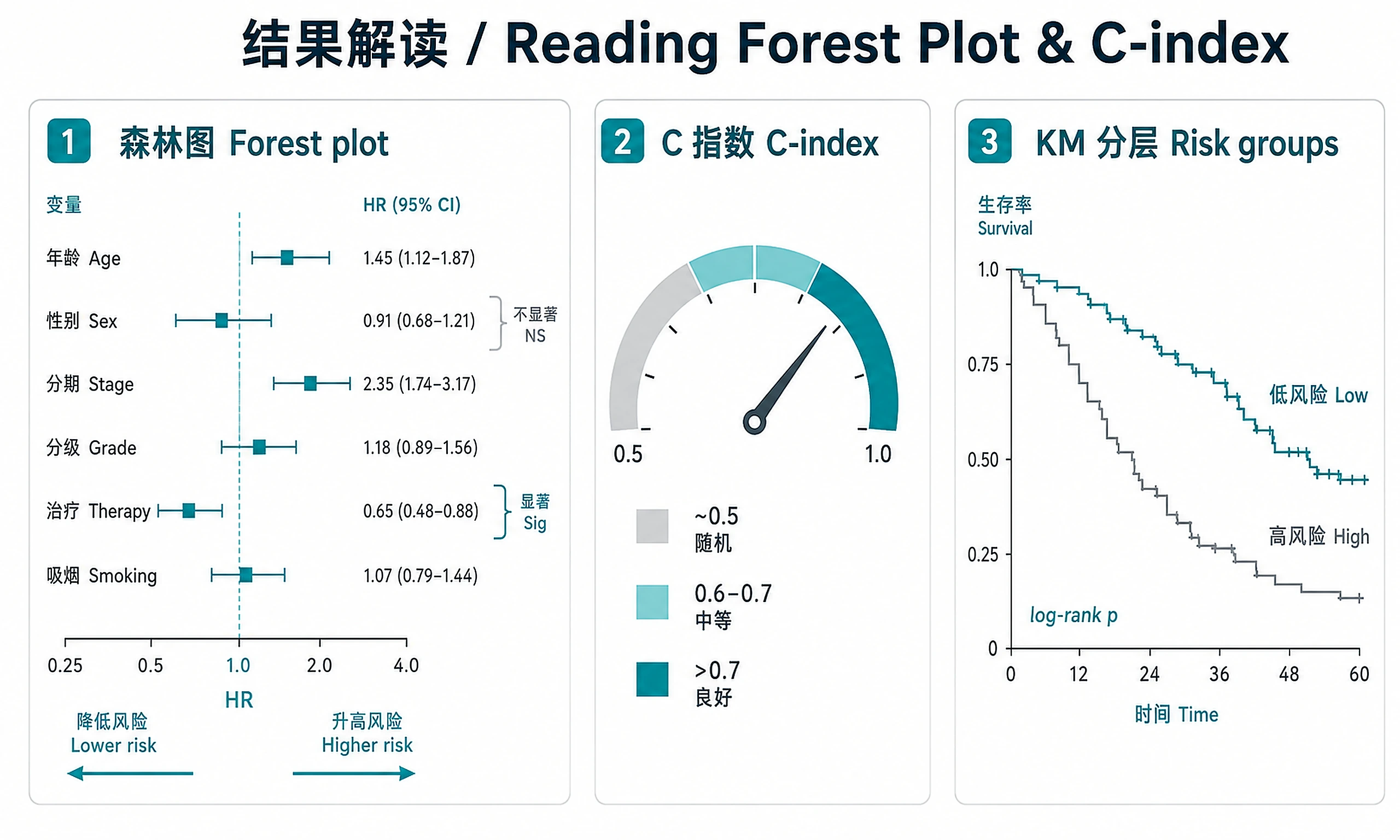
- Generate forest plots of hazard ratios for multi-covariate models
Don't use this skill for:
- ❌ Biomarker panel selection from omics → use
lasso-biomarker-panel - ❌ Differential expression analysis → use
bulk-rnaseq-counts-to-de-deseq2 - ❌ Disease trajectory / longitudinal modeling → use
disease-progression-longitudinal - ❌ Genetic association / Mendelian randomization → use
mendelian-randomization-twosamplemr
Installation
options(repos = c(CRAN = "https://cloud.r-project.org"))
if (!require('BiocManager', quietly = TRUE)) install.packages('BiocManager')

# Core (required)
install.packages(c('survival', 'ggplot2', 'ggprism', 'scales'))

# Enhanced KM curves with risk tables (recommended)
install.packages('survminer')

# Example data: TCGA BRCA (optional, needed for tcga_brca demo)
BiocManager::install('RTCGA.clinical')
| Software | Version | License | Commercial Use | Installation |
|---|---|---|---|---|
| survival | >=3.5 | LGPL (>=2) | ✅ Permitted | install.packages('survival') |
| ggplot2 | >=3.4 | MIT | ✅ Permitted | install.packages('ggplot2') |
| ggprism | >=1.0.3 | GPL (>=3) | ✅ Permitted | install.packages('ggprism') |
| scales | >=1.2 | MIT | ✅ Permitted | install.packages('scales') |
| survminer | >=0.4.9 | GPL (>=2) | ✅ Permitted | install.packages('survminer') |
Inputs
Required:
- Clinical data with columns for:
- Time-to-event (numeric: days, months, or years)
- Event indicator (binary: 0 = censored, 1 = event)
- Minimum 50 patients recommended (20+ events for reliable Cox estimates)
Optional:
- Stratification variable (e.g., molecular subtype, treatment arm, biomarker group)
- Covariates for Cox model (age, stage, receptor status, etc.)
- Pre-computed risk scores from upstream skills (e.g.,
lasso-biomarker-panel)
Formats: CSV/TSV with headers, or R data frame
Outputs
Primary results:
cox_coefficients.csv— Hazard ratios with 95% CI and p-values for all covariatesrisk_scores.csv— Patient-level risk scores and risk group assignmentsclinical_annotated.csv— Full clinical data with added risk group columnsurvival_summary.csv— Summary statistics per risk group (N, events, event rate, median survival)ph_assumption_test.csv— Schoenfeld residual test results (chi-sq, p-value per covariate)
Analysis objects (RDS):
survival_model.rds— Complete analysis object for downstream use- Load with:
model <- readRDS('results/survival_model.rds') - Contains: KM fits, Cox model, PH test, risk groups, clinical data, metadata
- Access risk scores:
model$cox$risk_scores - Access Cox model:
model$cox$model - Required for:
lasso-biomarker-panel(risk scores as features), downstream integration
Plots (PNG + SVG at 300 DPI):
km_overall.png/.svg— Overall Kaplan-Meier curve with confidence intervalkm_stratified.png/.svg— Stratified survival curves with log-rank p-valueforest_plot.png/.svg— Forest plot of hazard ratios with significance markerskm_risk_groups.png/.svg— Risk group survival curves with log-rank testschoenfeld_diagnostics.png/.svg— PH assumption diagnostic plotscumulative_hazard.png/.svg— Cumulative hazard function
Reports:
survival_report.md— Comprehensive markdown reportsurvival_report.pdf— Agent-generated PDF report with Introduction, Methods, Results, Conclusions, and embedded figures
⚠️ PDF style rules:
- US Letter page size (8.5 × 11 in) — always set page dimensions explicitly; do not rely on library defaults
- No Unicode superscripts — use
3.36e-06or3.36 × 10^(-6), not Unicode superscript chars (they render as ■ in PDF fonts) - No half-empty pages — group headings with their content; only page-break before major sections (Results, Conclusions)
- Figures ≥80% page width — multi-panel figures must be large enough to read; never embed below 50% width
Clarification Questions
🚨 ALWAYS ask Question 1 FIRST.
1. Example or Own Data? (ASK THIS FIRST):
- a) TCGA Breast Cancer (recommended for demo)
- 1,100+ patients with overall survival, molecular subtypes (HR+/HER2-, HR+/HER2+, HER2+, Triple Negative), stage, age, ER/PR/HER2 status
- Requires download (~50MB via RTCGA.clinical, cached after first run)
- b) NCCTG Lung Cancer (quick demo, no download)
- 228 advanced lung cancer patients, sex stratification, ECOG performance status
- Built-in R dataset — runs instantly
- c) I have my own clinical data to analyze
- Continue to Questions 2-3 below
IF EXAMPLE SELECTED (option a or b): Proceed to Question 2 for analysis options. Skip Question 3.
2. Analysis Options (structured — for all datasets):
- Stratification variable?
- a) Default for dataset (mol_subtype for TCGA BRCA, sex for Lung)
- b) Stage
- c) Age group
- Risk stratification method?
- a) Median split — 2 groups (recommended)
- b) Tertiles — 3 groups
- c) Quartiles — 4 groups
3. Data Details (own data only — free-text OK):
- What is the time column name? Units (days/months/years)?
- What is the event column name? What does 1 represent (death/relapse/progression)?
- What stratification variable? What covariates for the Cox model?
Standard Workflow
🚨 MANDATORY: USE SCRIPTS EXACTLY AS SHOWN - DO NOT WRITE INLINE CODE 🚨
Step 1 - Load data:
source("scripts/load_example_data.R")
data <- load_example_data(dataset = "tcga_brca")
# OR: data <- load_example_data(dataset = "lung")
# OR: data <- load_user_data("path/to/clinical.csv", time_col = "time", event_col = "status")
DO NOT write custom data loading code. Use the loader functions.
✅ VERIFICATION: You MUST see: "✓ TCGA BRCA data loaded successfully!" (or similar)
Step 2 - Run survival analysis:
source("scripts/basic_workflow.R")
result <- run_survival_analysis(data)
# Optional: result <- run_survival_analysis(data, risk_strata_method = "tertiles")
# Optional: result <- run_survival_analysis(data, covariates = c("age", "stage"))
DO NOT write inline Cox/KM code (coxph, survfit, etc.). Just source and call.
✅ VERIFICATION: You MUST see: "✓ Survival analysis completed successfully!"
❌ IF YOU DON'T SEE THIS: You wrote inline code. Stop and use source().
Step 3 - Generate visualizations:
source("scripts/survival_plots.R")
generate_all_plots(result, output_dir = "results")
DO NOT write inline plotting code (ggsave, ggplot, ggsurvplot, etc.). Just use generate_all_plots().
The script handles PNG + SVG export with graceful fallback for SVG dependencies.
✅ VERIFICATION: You MUST see: "✓ All survival plots generated successfully!"
Step 4 - Export results:
source("scripts/export_results.R")
export_all(result, output_dir = "results")
DO NOT write custom export code. Use export_all() to save all outputs including RDS.
✅ VERIFICATION: You MUST see:
"=== Export Complete ==="
⚠️ CRITICAL - DO NOT:
- ❌ Write inline Cox/KM code (coxph, survfit) → STOP: Use
source("scripts/basic_workflow.R") - ❌ Write inline plotting code (ggsave, ggplot, ggsurvplot) → STOP: Use
generate_all_plots() - ❌ Write custom export code → STOP: Use
export_all() - ❌ Try to install svglite → script handles SVG fallback automatically
⚠️ IF SCRIPTS FAIL - Script Failure Hierarchy:
- Fix and Retry (90%) - Install missing package, re-run script
- Modify Script (5%) - Edit the script file itself, document changes
- Use as Reference (4%) - Read script, adapt approach, cite source
- Write from Scratch (1%) - Only if genuinely impossible, explain why
NEVER skip directly to writing inline code without trying the script first.
Common Issues
| Error | Cause | Fix |
|---|---|---|
| "No valid covariates found" | All columns have >20% missing or single value | Provide covariates explicitly: run_survival_analysis(data, covariates = c("age", "stage")) |
| "Cox model failed with all covariates" | Collinear or non-convergent covariates | Script auto-falls back to stepwise. Inspect individual p-values. |
| PH assumption violated (global p < 0.05) | Time-varying effects | Note in report. Consider stratified analysis. See references/cox-regression-guide.md. |
| "Event column must be binary (0/1)" | Non-standard event coding | Recode: e.g., survival::lung uses 1=censored, 2=dead → script handles this. |
| RTCGA.clinical download fails | Network/firewall issue | Use dataset = "lung" as fallback (no download needed). |
| SVG export failed | Missing optional dependency | Normal — generate_all_plots() falls back automatically. PNG always generated. |
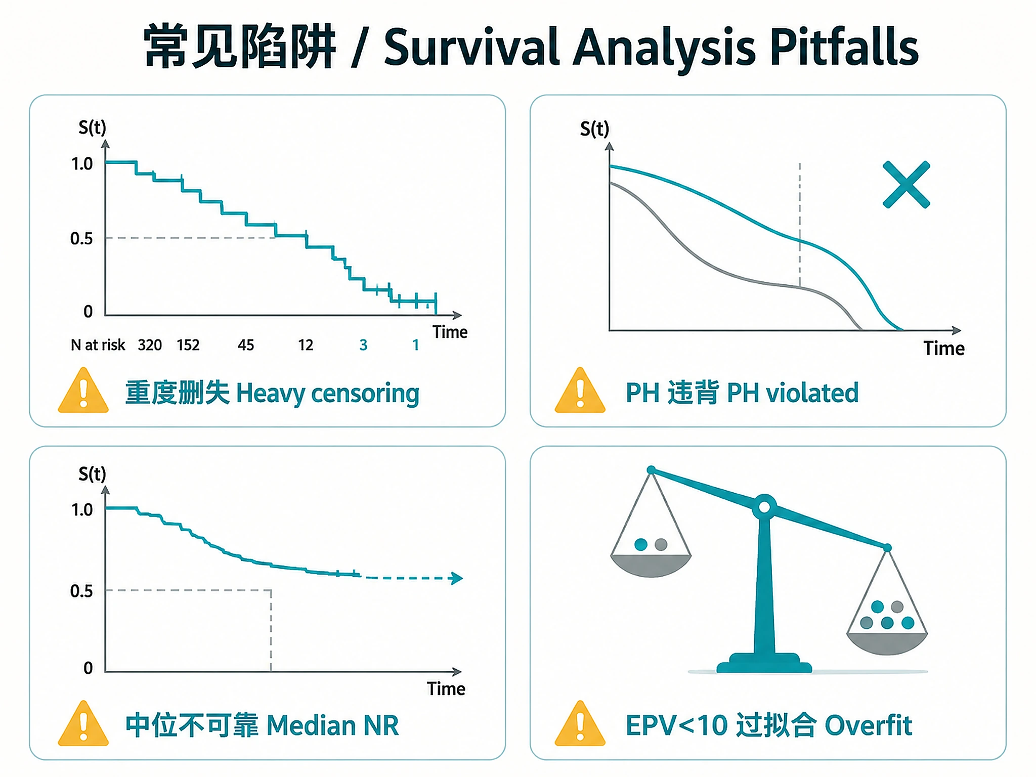
| KM curve drops steeply despite low event rate | Heavy censoring (correct behavior) | NOT A BUG. With heavy censoring (e.g., 90% censored), the at-risk set shrinks so each late event causes a large survival drop. The KM tail (N at risk < 30) is unreliable. Report landmark survival rates instead. |
| Subtype medians have upper CI = NA | KM never crosses 50% for that group | The median is an unreliable extrapolation. The script flags this — use landmark rates instead. Do NOT report these medians as reliable point estimates. |
Agent Summary Guidelines
When presenting final results to the user, the agent MUST:
- Report the C-index (concordance) from the Cox model — but see EPV rule below
- Check
result$median_reliable— if FALSE, report "Median survival: Not reached" and use landmark survival rates (fromresult$landmark_survival) instead - Report landmark survival rates (1-year, 3-year, 5-year OS with 95% CI) — these are always more robust than median, especially for low-event datasets
- State PH assumption result (satisfied or violated, with global p-value)
- List significant covariates with HR, 95% CI, and p-value
- Report EPV (events per variable) — if
result$epv < 10, warn that model may be overfitted - Report excluded patients — if
result$n_excluded > 0, note how many were excluded from Cox model - Report risk group separation (log-rank chi-sq and p-value)
- Report PDF status — if PDF generation failed, say so and note markdown report is available
- Never fabricate survival curve descriptions — reference the actual generated plots
- Never report unreliable medians as if they are reliable — when upper CI = NA, the KM curve did not cross 50% and the median is an unreliable extrapolation
- Methods section MUST match actual model — list only covariates from
names(coef(result$cox$model)). Checkresult$dropped_covariatesand report what was excluded and why. NEVER list covariates from memory; always verify against the fitted model. - Report dropped covariates — if
result$dropped_covariatesis non-empty, list each dropped variable and reason (rare levels, collinearity) in the Methods section - Report reference groups — for each categorical covariate, state the reference level and its N (from
result$reference_levels). If N < 50, flag the HR as "unstable due to small reference group (N=X)" - Report informative missingness — if any entry in
result$diagnostics$missing_assessmenthasinformative = TRUE, report the event rate comparison prominently and note selection bias risk - Report follow-up anomalies — if
result$diagnostics$followup_anomalyis TRUE, investigate and explain prominently. Do NOT dismiss as "expected" without evidence.
⚠️ CRITICAL REPORTING RULES:
- EPV < 10 + C-index: If
result$epv < 10, you MUST describe the C-index as "potentially overfitted" or "unreliable". NEVER use "good" or "moderate discrimination" without this caveat. The C-index is optimistically biased when EPV is low. - PH violation + forest plot/Cox table: If global PH test p < 0.05, you MUST include a prominent warning on the forest plot caption AND any Cox results table: "PH assumption violated (p=X) — HRs represent time-averaged effects and may be misleading." Do NOT present HRs as primary findings without this warning.
- Small reference groups: If a key finding involves a categorical covariate whose reference group has N < 50, flag the estimate as unstable. State the reference group N explicitly.
- Never fabricate group sizes or statistics. All Ns, HRs, CIs, and p-values in the report text MUST be copied from the script console output or exported CSV files. Do NOT estimate, round from memory, or recalculate group sizes. If a number is not in the output, re-run the relevant step or read the exported file.
Interpretation Guidelines
- C-index > 0.7: Good model discrimination — ONLY if EPV >= 10. If EPV < 10, say "potentially overfitted (EPV = X)"
- C-index 0.6-0.7: Moderate — useful combined with clinical factors
- C-index ~ 0.5: No better than chance
- HR > 1: Higher hazard (worse prognosis) per unit increase
- HR < 1: Lower hazard (protective effect)
- HR 95% CI includes 1.0: Not statistically significant
- PH global p < 0.05: Proportional hazards assumption violated — HRs are time-averaged and may be misleading. Must be stated prominently on forest plots and Cox tables, not buried in a later section.
- EPV < 10: Model underpowered — C-index likely optimistically biased; consider fewer covariates. NEVER call the C-index "good" when EPV < 10.
- Median survival "Not reached": KM curve never crosses 50% — use landmark survival rates instead
- Low event rate (<15%): KM curves may drop steeply in the tail due to small at-risk set (heavy censoring), not because most patients die. Always check N at risk at each timepoint.
- Median follow-up < 2 yr with max obs > 5 yr: Likely a data quality artifact — investigate completeness of follow-up times for censored patients before interpreting results.
Suggested Next Steps
- Biomarker panel discovery — Use risk scores as features →
lasso-biomarker-panel - Pathway enrichment — If molecular subtypes differ →
functional-enrichment-from-degs - Multi-omics integration — Combine clinical + omics →
multi-omics-integration-mofa - Disease trajectory — Map temporal progression →
disease-progression-longitudinal - Clinical trial landscape — Search related interventional trials →
clinicaltrials-landscape
Related Skills
| Skill | Relationship |
|---|---|
lasso-biomarker-panel |
Downstream — Use risk scores as features for biomarker selection |
disease-progression-longitudinal |
Complementary — Trajectory analysis on same clinical data |
multi-omics-integration-mofa |
Upstream — Factor scores as Cox covariates |
bulk-rnaseq-counts-to-de-deseq2 |
Upstream — DE results inform covariate selection |
coexpression-network |
Upstream — Module eigengenes as survival predictors |
References
- Cox DR. Regression Models and Life-Tables. J R Stat Soc B. 1972;34(2):187-220.
- Kaplan EL, Meier P. Nonparametric Estimation from Incomplete Observations. JASA. 1958;53(282):457-481.
- Cancer Genome Atlas Network. Comprehensive molecular portraits of human breast tumours. Nature. 2012;490:61-70.
- Loprinzi CL, et al. Prospective evaluation of prognostic variables from patient-completed questionnaires. J Clin Oncol. 1994;12:601-607.
- Therneau TM. A Package for Survival Analysis in R. R package survival.
- See references/cox-regression-guide.md for detailed Cox PH interpretation
- See references/risk-stratification-guide.md for risk group methodology
Code preview
scripts/basic_workflow.R
# =============================================================================
# Survival Analysis Workflow
# =============================================================================
# Core functions for Cox proportional hazards analysis, Kaplan-Meier estimation,
# risk stratification, and assumption testing.
#
# Usage:
#   source("scripts/basic_workflow.R")
#   result <- run_survival_analysis(data)
# =============================================================================

library(survival)

# =============================================================================
# Main Entry Point
# =============================================================================

run_survival_analysis <- function(data, covariates = NULL,
                                  risk_strata_col = NULL,
                                  risk_strata_method = "median") {
    cat("\n=== Running Survival Analysis ===\n\n")

    clinical <- data$clinical
    event_col <- data$event_col
    time_col <- data$time_col
    strata_col <- data$strata_col

    # --- Validate ---
    .validate_survival_data(clinical, event_col, time_col)

    # --- 1. Kaplan-Meier estimation (overall) ---
    cat("1. Kaplan-Meier estimation (overall)...\n")
    km_formula <- as.formula(paste0("Surv(", time_col, ", ", event_col, ") ~ 1"))
    km_overall <- survfit(km_formula, data = clinical)
    median_surv <- summary(km_overall)$table["median"]
    median_reliable <- .median_is_reliable(km_overall)

    # Landmark survival rates (robust even when median is unreliable)
    max_time <- max(clinical[[time_col]], na.rm = TRUE)
    landmark_times <- if (max_time > 3) c(1, 3, 5) else c(0.5, 1, 2)
    landmark_times <- landmark_times[landmark_times < max_time]
    landmark_surv <- .compute_landmark_survival(km_overall, landmark_times)

    # Median follow-up (reverse KM — standard method)
    median_followup <- .compute_median_followup(clinical, time_col, event_col)

    event_rate <- mean(clinical[[event_col]])
    n_censored <- sum(clinical[[event_col]] == 0)
    pct_censored <- round(100 * n_censored / nrow(clinical), 1)

    cat("   Events:", sum(clinical[[event_col]]), "/", nrow(clinical),
        "(", round(100 * event_rate, 1), "% event rate)\n")
    cat("   Censored:", n_censored, "/", nrow(clinical),
        "(", pct_censored, "%)\n")
    cat("   Median follow-up (reverse KM):", round(median_followup, 2), "years\n")

    # Heavy censoring warning — explains why KM curve may drop steeply in the tail
    if (event_rate < 0.20 && pct_censored > 80) {
        cat("\n   NOTE: HEAVY CENSORING DETECTED (", pct_censored,
            "% censored, ", round(100 * event_rate, 1), "% event rate)\n", sep = "")
        cat("   The KM curve may drop steeply in the tail despite a low overall event rate.\n")
        cat("   This is mathematically correct: as patients are censored, the at-risk set\n")
        cat("   shrinks, so each late event causes a larger survival drop. The tail of the\n")
        cat("   curve (where N at risk is small) is UNRELIABLE. Use landmark survival rates.\n")
    }

    if (median_reliable) {
        cat("   Median survival:", round(median_surv, 2), "years\n")
    } else {
        cat("   Median survival: NOT REACHED (KM curve does not cross 50%)\n")
    }

    # Always show landmark survival for transparency
    cat("   Landmark survival rates:\n")
    for (i in seq_len(nrow(landmark_surv))) {
        cat(sprintf("     %g-year OS: %.1f%% (95%% CI: %.1f%%-%.1f%%), n at risk: %d\n",
            landmark_surv$time[i],
            100 * landmark_surv$survival[i],
            100 * landmark_surv$lower_ci[i],
            100 * landmark_surv$upper_ci[i],
scripts/export_results.R
# =============================================================================
# Export Survival Analysis Results
# =============================================================================
# Exports all results: CSVs, RDS objects, summary tables, and PDF report.
#
# Usage:
#   source("scripts/export_results.R")
#   export_all(result, output_dir = "results")
# =============================================================================

export_all <- function(result, output_dir = "results") {
    cat("\n=== Exporting Survival Analysis Results ===\n\n")

    if (!dir.exists(output_dir)) dir.create(output_dir, recursive = TRUE)

    # --- 1. Cox model coefficients ---
    cat("1. Cox model coefficients...\n")
    coef_out <- result$cox$coefficients
    # Remove reference level rows (NA coefficients) for clean output
    coef_out <- coef_out[!is.na(coef_out$pval), ]
    write.csv(coef_out,
              file.path(output_dir, "cox_coefficients.csv"),
              row.names = FALSE)
    cat("   Saved: cox_coefficients.csv\n\n")

    # --- 2. Patient risk scores ---
    cat("2. Patient risk scores...\n")
    scores_df <- data.frame(
        sample_id = result$clinical$sample_id,
        risk_score = result$cox$risk_scores,
        risk_group = result$clinical[[result$risk_col]],
        stringsAsFactors = FALSE
    )
    write.csv(scores_df, file.path(output_dir, "risk_scores.csv"),
              row.names = FALSE)
    cat("   Saved: risk_scores.csv\n\n")

    # --- 3. Clinical data with risk groups ---
    cat("3. Annotated clinical data...\n")
    write.csv(result$clinical,
              file.path(output_dir, "clinical_annotated.csv"),
              row.names = FALSE)
    cat("   Saved: clinical_annotated.csv\n\n")

    # --- 4. Survival summary table ---
    cat("4. Survival summary statistics...\n")
    summary_df <- .build_summary_table(result)
    write.csv(summary_df, file.path(output_dir, "survival_summary.csv"),
              row.names = FALSE)
    cat("   Saved: survival_summary.csv\n\n")

    # --- 5. PH assumption test ---
    cat("5. Proportional hazards test results...\n")
    ph_df <- data.frame(
        variable = rownames(result$ph_test$table),
        chisq = result$ph_test$table[, "chisq"],
        df = result$ph_test$table[, "df"],
        p = result$ph_test$table[, "p"],
        stringsAsFactors = FALSE,
        row.names = NULL
    )
    write.csv(ph_df, file.path(output_dir, "ph_assumption_test.csv"),
              row.names = FALSE)
    cat("   Saved: ph_assumption_test.csv\n\n")

    # --- 6. Analysis object (RDS) - CRITICAL for downstream skills ---
    cat("6. Saving analysis object (RDS)...\n")
    saveRDS(result, file.path(output_dir, "survival_model.rds"))
    cat("   Saved: survival_model.rds\n")
    cat("   (Load with: model <- readRDS('results/survival_model.rds'))\n\n")

    # --- 7. Markdown report ---
    cat("7. Generating markdown report...\n")
    md_content <- .build_markdown_report(result)
    writeLines(md_content, file.path(output_dir, "survival_report.md"))
    cat("   Saved: survival_report.md\n\n")

    cat("\n=== Export Complete ===\n")
    cat("\nFiles in", output_dir, ":\n")
    files <- list.files(output_dir, recursive = FALSE)
scripts/load_example_data.R
# =============================================================================
# Load Example Data for Survival Analysis
# =============================================================================
# Provides two example datasets:
#   1. TCGA BRCA (breast cancer) - Real-world clinical data with molecular markers
#   2. NCCTG Lung - Built-in survival::lung dataset (no download needed)
# =============================================================================

options(repos = c(CRAN = "https://cloud.r-project.org"))

# --- Helper: ensure Bioconductor package installed ---
.ensure_bioc_package <- function(pkg) {
    if (!requireNamespace(pkg, quietly = TRUE)) {
        if (!requireNamespace("BiocManager", quietly = TRUE)) {
            install.packages("BiocManager")
        }
        cat("  Installing", pkg, "...\n")
        BiocManager::install(pkg, ask = FALSE, update = FALSE)
    }
}

# =============================================================================
# Option 1: TCGA Breast Cancer (BRCA) - Real-World Clinical Data
# =============================================================================
# Source: The Cancer Genome Atlas via RTCGA.clinical
# ~1,100 patients with overall survival, stage, ER/PR/HER2 status
# Clear survival differences by stage and receptor status
# =============================================================================

load_tcga_brca <- function(data_dir = "data") {
    cat("\n=== Loading TCGA BRCA Survival Data ===\n\n")

    if (!dir.exists(data_dir)) dir.create(data_dir, recursive = TRUE)

    # Check cache
    cache_file <- file.path(data_dir, "tcga_brca_survival.rds")
    if (file.exists(cache_file)) {
        cat("  Loading from cache...\n")
        data <- readRDS(cache_file)
        cat("✓ TCGA BRCA data loaded successfully!\n")
        cat("  Samples:", nrow(data$clinical), "\n")
        cat("  Events:", sum(data$clinical$event, na.rm = TRUE), "\n")
        return(data)
    }

    # Install RTCGA.clinical if needed
    .ensure_bioc_package("RTCGA.clinical")

    cat("  Extracting BRCA clinical data...\n")
    library(RTCGA.clinical)
    data("BRCA.clinical", package = "RTCGA.clinical", envir = environment())

    raw <- BRCA.clinical

    # --- Extract and clean survival variables ---

    # Vital status: alive=0, dead=1
    vital <- tolower(trimws(raw$patient.vital_status))
    event <- ifelse(vital == "dead", 1L, 0L)

    # Survival time in days -> years
    days_death <- suppressWarnings(as.numeric(raw$patient.days_to_death))
    days_fu <- suppressWarnings(as.numeric(raw$patient.days_to_last_followup))
    time_days <- ifelse(!is.na(days_death) & event == 1, days_death, days_fu)
    time_years <- time_days / 365.25

    # Age at diagnosis
    age <- suppressWarnings(
        as.numeric(raw$patient.age_at_initial_pathologic_diagnosis)
    )

    # Pathologic stage (simplify to I-IV)
    stage_raw <- tolower(trimws(raw$patient.stage_event.pathologic_stage))
    stage <- case_when_stage(stage_raw)

    # Receptor status
    er_status <- clean_receptor(
        raw$patient.breast_carcinoma_estrogen_receptor_status
    )
    pr_status <- clean_receptor(
Companion files
| Type | Path | Bytes |
|---|---|---|
| Markdown | references/cox-regression-guide.md | 5,210 |
| Markdown | references/risk-stratification-guide.md | 2,198 |
| R | scripts/basic_workflow.R | 26,276 |
| R | scripts/export_results.R | 12,237 |
| R | scripts/load_example_data.R | 12,913 |
| R | scripts/survival_plots.R | 15,988 |
| Markdown | SKILL.md | 16,536 |
| JSON | skill.meta.json | 1,827 |