Omics Clustering
Cluster samples or genes to find subtypes, with rigorous k-selection.

Overview
Problem. Find natural groupings and compare clustering methods.
Learning goals
- k is chosen systematically, not by guess
- Trust clusters that survive resampling
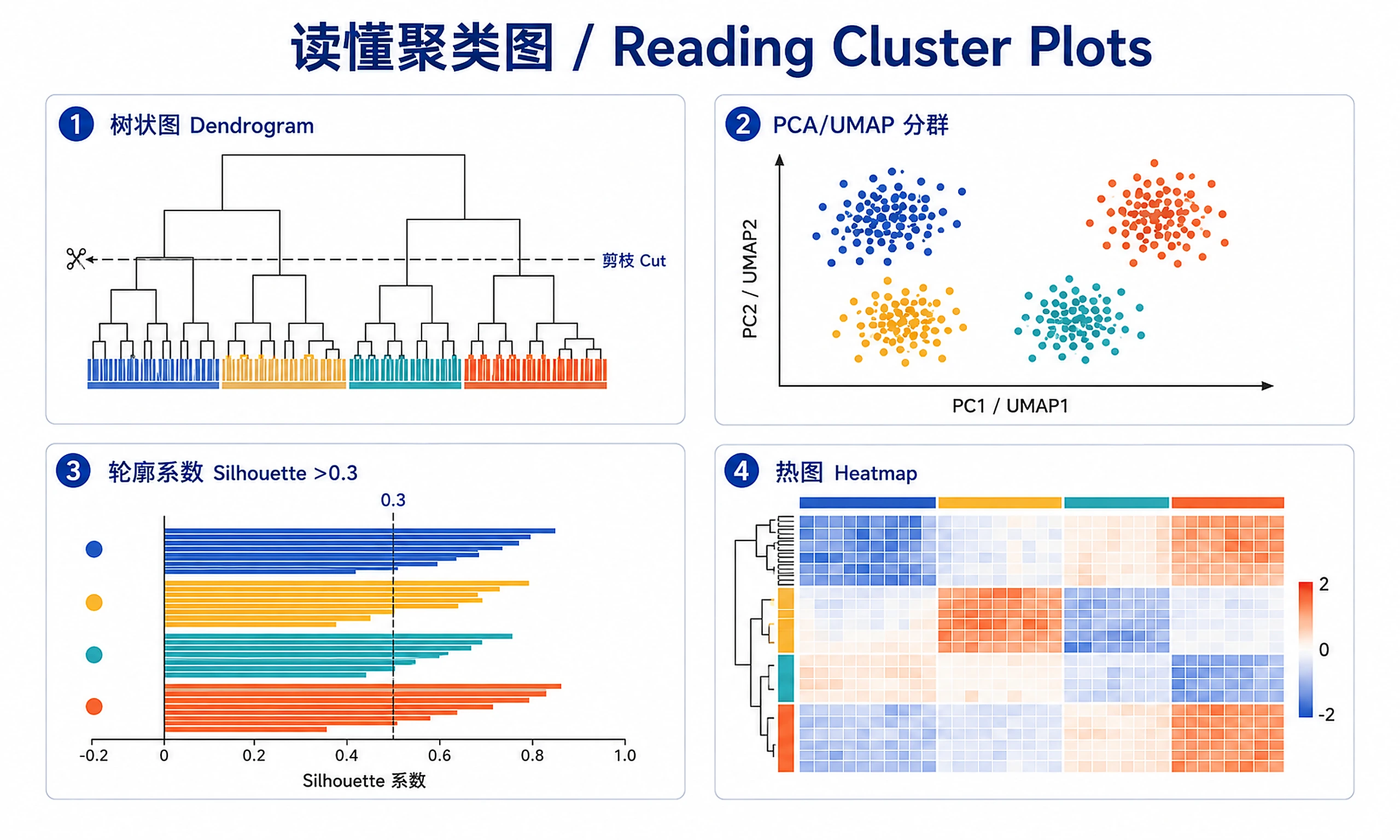
Figures

Tutorial
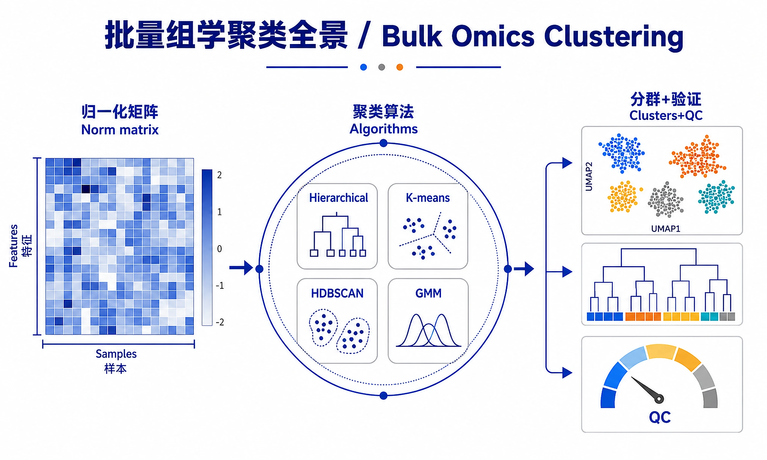
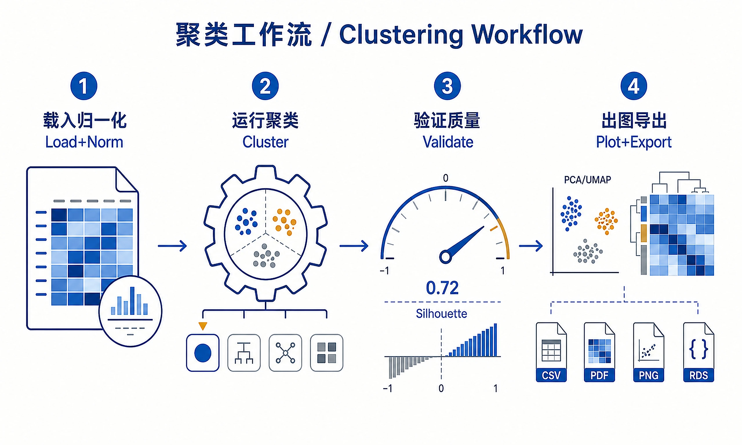
Systematic workflow for clustering biological samples, features, or any quantitative data matrix. Implements multiple clustering algorithms with rigorous validation, comparison, and interpretation to identify meaningful data groupings.
When to Use This Skill
Use clustering analysis when you need to:
- ✅ Group biological samples by gene expression profiles (bulk RNA-seq, proteomics)
- ✅ Identify feature patterns (genes/proteins with similar expression across conditions)
- ✅ Discover subtypes in disease or treatment response groups
- ✅ Analyze trajectories in time-series or developmental data
- ✅ Quality control by detecting batch effects or outliers
- ✅ Compare methods by systematically evaluating multiple clustering approaches
Don't use this skill for:
- ❌ Single-cell RNA-seq clustering → Use scrnaseq-scanpy-core-analysis or scrnaseq-seurat-core-analysis
- ❌ Gene co-expression network analysis → Use coexpression-network
Key Concept: Clustering reveals natural groupings in data without prior labels. Different algorithms make different assumptions—this workflow helps you choose and validate the right approach for your data.
Language Support: This skill supports both Python and R implementations. Choose based on your preference and existing analysis pipeline. Python offers scikit-learn ecosystem integration; R offers ComplexHeatmap and rich Bioconductor tools.
Quick Start (5-Minute Example)
Test the workflow with the ALL (Acute Lymphoblastic Leukemia) dataset - 128 pediatric ALL patients with B-cell and T-cell subtypes:
R (Recommended for ALL dataset):
# 1. Load example data (ALL dataset from Chiaretti et al. 2004)
source("scripts/load_example_data.R")
data_list <- load_example_clustering_data()
data <- data_list$data
sample_names <- data_list$sample_names
feature_names <- data_list$feature_names
metadata <- data_list$metadata

# 2. Run clustering
source("scripts/hierarchical_clustering.R")
result <- hierarchical_clustering(data, n_clusters = 2)
cluster_labels <- result$cluster_labels
hclust_obj <- result$clustering_object

# 3. Visualize
source("scripts/plot_cluster_heatmap.R")
plot_cluster_heatmap(
  data,
  cluster_labels,
  output_dir = "quick_test_results"
)

# 4. Export results
# Results automatically saved by plotting functions
cat("\n✓ Quick start complete!\n")
cat(sprintf("Cell types: B-cell ALL (n=%d), T-cell ALL (n=%d)\n",
            sum(metadata$cell_type == "B"),
            sum(metadata$cell_type == "T")))
Python users: The Python implementation can use the same ALL dataset via rpy2, or use your own data. For ALL dataset examples in Python, you'll need pip install rpy2 and R installed. See full workflow below.
Expected output: Dendrogram distinguishing B-cell vs T-cell ALL, PCA plots, silhouette plots, heatmaps in quick_test_results/
Note: For your own data, follow the full workflow below with the Clarification Questions.
Installation
Language Choice
This workflow supports both Python and R. Choose one based on:
- Python: Better for large-scale data (>10k samples), integration with machine learning pipelines, modern plotting (plotnine)
- R: Better for heatmap visualization (ComplexHeatmap), Bioconductor integration, traditional bioinformatics workflows
You can also mix: use R for visualization (heatmaps) and Python for clustering algorithms.
Python Installation
Required Software
| Software | Version | License | Commercial Use | Installation |
|---|---|---|---|---|
| numpy | ≥1.20 | BSD-3-Clause | ✅ Permitted | pip install numpy |
| pandas | ≥1.3 | BSD-3-Clause | ✅ Permitted | pip install pandas |
| scikit-learn | ≥1.0 | BSD-3-Clause | ✅ Permitted | pip install scikit-learn |
| scipy | ≥1.7 | BSD-3-Clause | ✅ Permitted | pip install scipy |
| hdbscan | ≥0.8.28 | BSD-3-Clause | ✅ Permitted | pip install hdbscan |
| umap-learn | ≥0.5 | BSD-3-Clause | ✅ Permitted | pip install umap-learn |
| plotnine | ≥0.10 | MIT | ✅ Permitted | pip install plotnine |
| plotnine-prism | Latest | MIT | ✅ Permitted | pip install plotnine-prism |
| seaborn | ≥0.11 | BSD-3-Clause | ✅ Permitted | pip install seaborn |
| matplotlib | ≥3.4 | PSF-based | ✅ Permitted | pip install matplotlib |
| adjustText | ≥0.8 | MIT | ✅ Permitted | pip install adjustText |
| statsmodels | ≥0.13 | BSD-3-Clause | ✅ Permitted | pip install statsmodels |
Optional: gap-stat (Apache 2.0), yellowbrick (Apache 2.0) - both permitted for commercial use
Minimum Python version: Python ≥3.8
License Compliance: All software packages use BSD-3-Clause, MIT, or similar permissive licenses that allow commercial use in AI agent applications.
R Installation
Minimum R version: R ≥4.0
Required packages: cluster, factoextra, NbClust, ComplexHeatmap, pheatmap, dendextend, dbscan, mclust, ggplot2, ggprism (all GPL/MIT licensed, commercial use permitted)
Quick install:
install.packages(c('cluster', 'factoextra', 'NbClust', 'pheatmap',
                   'dendextend', 'dbscan', 'mclust', 'ggplot2', 'ggprism'))
if (!require('BiocManager')) install.packages('BiocManager')
BiocManager::install('ComplexHeatmap')
Detailed R installation guide: references/r-quick-start.md#r-installation
Inputs
Required Input
1. Data Matrix (CSV, TSV, Excel, or HDF5):
- Sample clustering: Rows = samples, Columns = features (genes/proteins)
- Feature clustering: Rows = features, Columns = samples
- Values should be normalized and comparable (TPM, FPKM, VST, Z-scores)
- Missing values: handle by imputation or removal before clustering
2. Sample/Feature Metadata (CSV or TSV, optional but recommended):
- IDs matching data matrix rows/columns
- Annotations for validation (tissue type, condition, known groups)
- Used to interpret and validate clustering results
Data Requirements
- Minimum samples/features: 10+ (20+ recommended for robust clustering)
- Normalization: Required—use appropriate method for data type
- Batch effects: Remove or regress out before clustering
- Outliers: Identify and consider removing extreme outliers
- Dimensionality: High-dimensional data (>1000 features) benefits from PCA first
Supported Data Types
- Transcriptomics: Bulk RNA-seq (normalized counts, TPM, FPKM)
- Proteomics: Protein abundance data
- Metabolomics: Metabolite concentrations
- Multi-omics: Integrated features from multiple assays
- Clinical: Patient feature matrices
- Any quantitative matrix: General-purpose application
Outputs
Cluster assignments:
clustering_assignments.csv- Sample/feature IDs with cluster labelsclustering_statistics.csv- Size, centroids, and characteristics per cluster
Validation metrics:
clustering_validation_metrics.json- Silhouette, Davies-Bouldin, Calinski-Harabasz scoresstability_results.csv- Bootstrap resampling stability scores (if run)
Characterization:
clustering_cluster*_features.csv- Top distinguishing features for each cluster (ANOVA/Kruskal-Wallis)clustering_all_cluster_features.csv- Combined features for all clusters
Analysis objects (pickle/RDS):
clustering_analysis_object.pkl- Complete clustering object for downstream use- Load with:
import pickle; obj = pickle.load(open('clustering_analysis_object.pkl', 'rb')) - Contains: linkage matrix (hierarchical), fitted model (k-means, GMM, HDBSCAN)
- Required for: Advanced analysis, re-cutting dendrograms, model inspection
clustering_data_matrix.csv- Normalized/transformed data matrix used for clustering
Visualizations (PNG + SVG at 300 DPI):
- Dendrogram (hierarchical clustering)
- PCA/UMAP scatter plots with cluster colors
- Silhouette plots
- Cluster heatmaps
- Cluster size barplots
- Optimal k determination plots (if run)
Supporting data:
clustering_parameters.json- All parameters used in analysis
Clarification Questions
Before starting analysis, gather the following information:
1. Input Files (ASK THIS FIRST):
- Do you have specific gene expression or omics data file(s) to cluster?
- If you've uploaded a file, is it the data matrix (samples × features or features × samples) you'd like to analyze?
- Expected file types: CSV, TSV, Excel (.xlsx), HDF5 (.h5), or RDS (R data objects)
- Or use ALL (Acute Lymphoblastic Leukemia) example data? (Real patient data: 128 pediatric ALL samples with B-cell and T-cell subtypes, 1000 most variable genes. Dynamically loads from Bioconductor in ~30 seconds via scripts/load_example_data.R. Citation: Chiaretti et al. 2004. R recommended for this dataset.)
2. Which programming language do you prefer?
- Python: Modern ecosystem with scikit-learn, better for large datasets (>10k samples), machine learning integration
- R: Rich Bioconductor tools, excellent heatmap visualization (ComplexHeatmap), traditional bioinformatics workflows
- Both: Use Python for clustering algorithms, R for heatmap visualization (recommended for best of both worlds)
- No preference: Will use Python (default, more comprehensive scripts available)
3. What are you clustering?
- Samples (rows = samples, columns = features like genes)
- Example: Group patients by gene expression profiles
- Features (rows = features, columns = samples)
- Example: Group genes by expression patterns across conditions
- Both (explore both clustering directions)
4. What is your data format and normalization status?
- Bulk RNA-seq: TPM, FPKM, VST, rlog
- Proteomics: TMT/iTRAQ normalized intensities, LFQ
- Metabolomics: Normalized peak areas
- Already normalized: Z-scores, scaled values
- Raw data: Needs normalization (specify data type)
5. What clustering approach do you prefer?
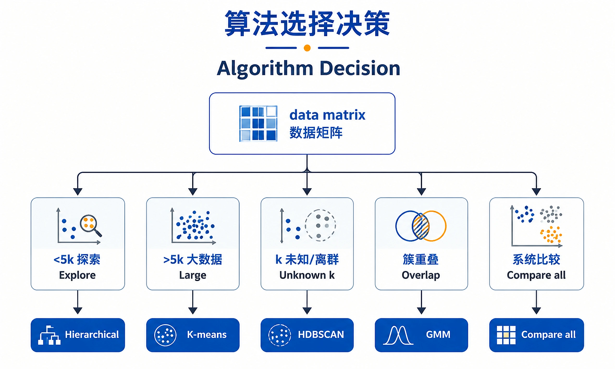
- Hierarchical (recommended for exploration): Creates a tree-like dendrogram showing relationships at all scales. You can cut the tree at any height to get different numbers of clusters after seeing the structure. Best for visualization and when you don't know k. Deterministic (same results every run). Works well for small-medium datasets (<5k samples).
- K-means: Fast partitioning method that requires specifying k upfront. Best for large datasets (>5k samples) with spherical/compact clusters. Results may vary between runs, so use high n_init.
- Density-based (HDBSCAN): Automatically finds k by identifying dense regions. Can detect arbitrary cluster shapes and marks outliers. No need to specify k. Best when clusters have varying densities or you want outlier detection.
- Model-based (GMM): Probabilistic soft clustering where samples have membership probabilities for each cluster. Useful when clusters overlap or you need uncertainty estimates. Requires specifying k.
- Compare all methods: Systematic comparison (recommended for exploratory analysis)
6. Do you know the expected number of clusters (k)?
- Yes, k = [number]: Will validate this choice with quality metrics
- No, exploratory: Will test multiple k values (2-15) and help determine optimal k
- Approximate range: k between [min] and [max]
- Not needed: Hierarchical clustering lets you choose k later; HDBSCAN finds k automatically
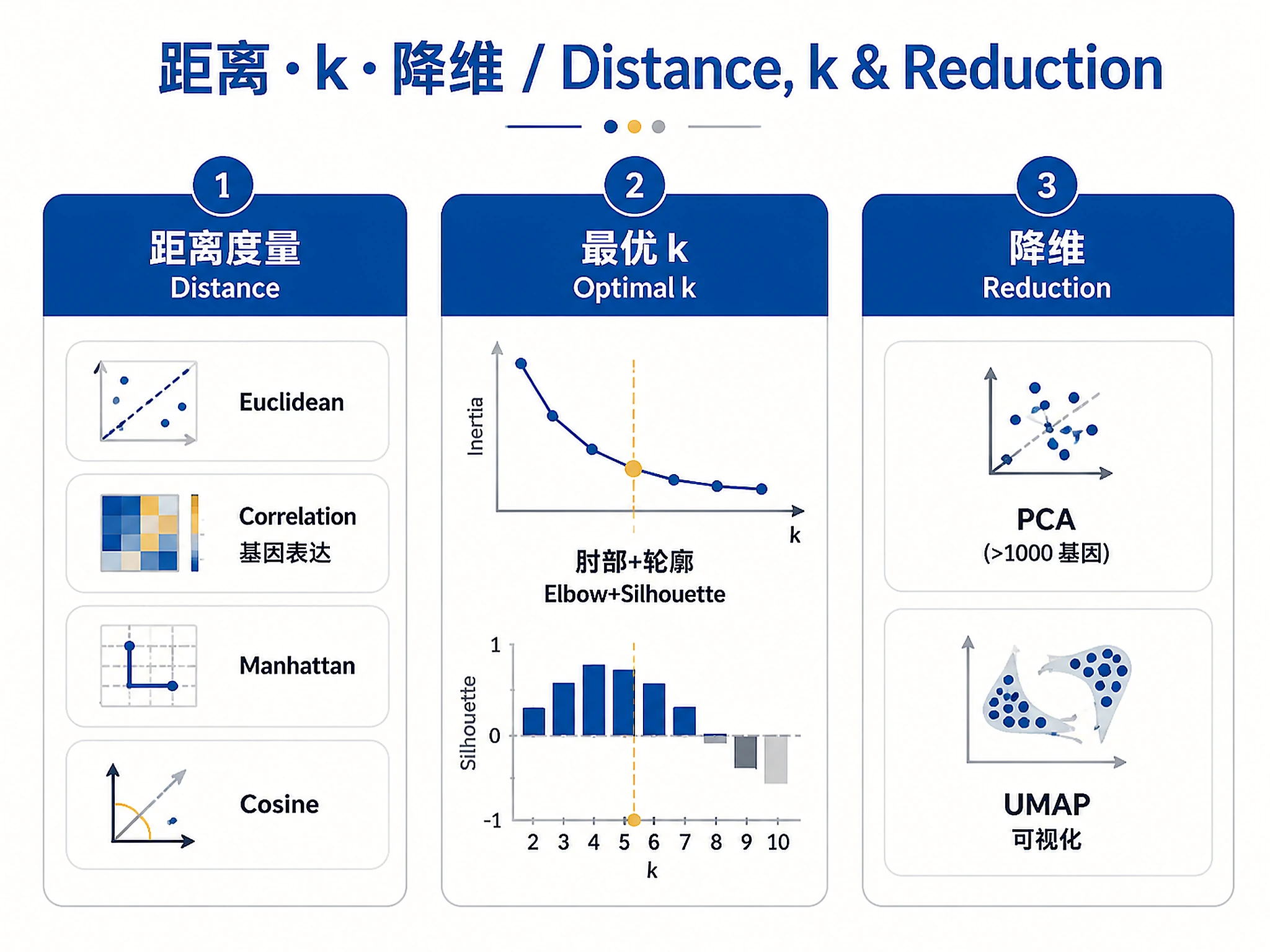
7. What distance metric is most appropriate?
- Euclidean: Default for most continuous data
- Correlation: For gene expression (focuses on pattern similarity)
- Manhattan: Robust to outliers
- Cosine: For high-dimensional sparse data
- Unsure: Will use Euclidean (default)
8. Should we apply dimensionality reduction first?
- Yes, use PCA: Recommended for >1000 features
- Yes, use UMAP: For visualization and manifold learning
- No: Keep original feature space (<100 features)
- Both: PCA for clustering, UMAP for visualization
9. How should cluster quality be validated?
- Internal metrics only: Silhouette, Davies-Bouldin, Calinski-Harabasz
- Known labels available: Compare to known groups (adjusted Rand index)
- Stability analysis: Bootstrap resampling to test robustness
- Biological validation: Check for differential features between clusters
Standard Workflow
🚨 MANDATORY: USE SCRIPTS EXACTLY AS SHOWN - DO NOT WRITE INLINE CODE 🚨
Note: This skill requires decisions (algorithm, distance metric, k value) - adapt parameters to your data using guidance in references/decision-guide.md.
Step 1 - Load data:
For ALL example data (R recommended):
source("scripts/load_example_data.R")
data_list <- load_example_clustering_data()
data <- data_list$data
sample_names <- data_list$sample_names
feature_names <- data_list$feature_names
metadata <- data_list$metadata
For your own data (Python or R):
# Python
from scripts.prepare_data import load_and_prepare_data
data, sample_names, feature_names = load_and_prepare_data(
    "your_data.csv",
    normalize_method="zscore"
)
# R
source("scripts/prepare_data.R")
data_list <- load_and_prepare_data("your_data.csv", normalize_method = "zscore")
data <- data_list$data
DO NOT write custom data loading code. Use the provided functions.
Step 2 - Run clustering analysis:
# Choose ONE clustering method and run it:

# Option A: Hierarchical clustering (recommended for exploration)
from scripts.hierarchical_clustering import hierarchical_clustering
linkage_matrix, cluster_labels = hierarchical_clustering(
    data,
    n_clusters=2,  # For ALL dataset: B-cell vs T-cell; adjust for your data
    linkage_method="ward",
    distance_metric="euclidean"
)
clustering_object = linkage_matrix

# Option B: K-means clustering (fast, for large datasets)
from scripts.kmeans_clustering import kmeans_clustering
cluster_labels, kmeans_model = kmeans_clustering(
    data,
    n_clusters=2,  # For ALL dataset: B-cell vs T-cell; adjust for your data
    n_init=50
)
clustering_object = kmeans_model

# Option C: HDBSCAN (automatic k detection)
from scripts.density_clustering import hdbscan_clustering
cluster_labels, hdbscan_model = hdbscan_clustering(
    data,
    min_cluster_size=10
)
clustering_object = hdbscan_model

# Validate clustering quality
from scripts.cluster_validation import validate_clustering
validation_results = validate_clustering(data, cluster_labels, metrics="all")
print(f"Silhouette score: {validation_results['silhouette']:.3f}")
DO NOT write custom clustering code. Use one of the provided methods.
Step 3 - Generate visualizations:
# Generate comprehensive plots
from scripts.plot_clustering_results import plot_all_results
from scripts.dimensionality_reduction import apply_pca, apply_umap

# Optional: compute PCA/UMAP for visualization
pca_data = apply_pca(data, n_components=2)
umap_data = apply_umap(data, n_components=2)

# Create all plots
plot_all_results(
    data=data,
    cluster_labels=cluster_labels,
    sample_names=sample_names,
    feature_names=feature_names,
    pca_data=pca_data,
    umap_embedding=umap_data,
    linkage_matrix=clustering_object if 'linkage_matrix' in locals() else None,
    output_dir="clustering_results"
)
DO NOT write inline plotting code (matplotlib.pyplot.savefig, seaborn.clustermap, etc.). Use plot_all_results().
The script handles PNG + SVG export with graceful fallback for optional dependencies.
Step 4 - Export results:
# Export all results including analysis objects for downstream use
from scripts.export_results import export_all

export_all(
    data=data,
    cluster_labels=cluster_labels,
    sample_names=sample_names,
    feature_names=feature_names,
    validation_results=validation_results,
    clustering_object=clustering_object,
    output_dir="clustering_results"
)
DO NOT write custom export code. Use export_all().
✅ VERIFICATION - You should see:
- After Step 1:
"✓ Data loaded successfully!" - After Step 2:
"✓ Clustering completed successfully!" - After Step 3:
"✓ Plots saved to clustering_results" - After Step 4:
"=== Export Complete ==="
❌ IF YOU DON'T SEE THESE: You wrote inline code. Stop and use the scripts as shown.
⚠️ CRITICAL - DO NOT:
- ❌ Write inline clustering algorithms → STOP: Use provided clustering functions
- ❌ Write inline plotting code (matplotlib.pyplot.savefig, seaborn.clustermap, etc.) → STOP: Use
plot_all_results() - ❌ Write custom export code → STOP: Use
export_all() - ❌ Try to install plotting dependencies manually → scripts handle fallback automatically
⚠️ IF SCRIPTS FAIL - Script Failure Hierarchy:
- Fix and Retry (90%) - Install missing package, re-run script
- Modify Script (5%) - Edit the script file itself, document changes
- Use as Reference (4%) - Read script, adapt approach, cite source
- Write from Scratch (1%) - Only if genuinely impossible, explain why
NEVER skip directly to writing inline code without trying the script first.
For detailed parameter guidance and decision-making, see:
- Algorithm selection: references/decision-guide.md#algorithm
- Distance metrics: references/decision-guide.md#distance
- Optimal k: references/decision-guide.md#optimal-k
Common Issues
| Error | Cause | Solution |
|---|---|---|
ValueError: n_clusters exceeds n_samples |
Too many clusters requested for dataset size | Reduce k or ensure data has ≥10 samples |
Ward linkage requires euclidean distance |
Incompatible linkage method and distance metric | Use euclidean distance with ward, or switch to average/complete linkage |
ModuleNotFoundError: No module named 'plotnine_prism' |
Missing optional visualization dependency | Install: pip install plotnine-prism |
| Silhouette score < 0.25 | Poor cluster separation, k may be wrong | Try different k values, check data quality, use optimal k methods |
| HDBSCAN returns only noise (-1 labels) | min_cluster_size too large for dataset | Reduce min_cluster_size (try 5-10 for small datasets) or increase min_samples |
ValueError: Input contains NaN |
Missing values in data matrix | Impute or remove NaN values before clustering |
| Clusters of very unequal sizes | Algorithm bias or true biological structure | Validate with biology; try HDBSCAN for density-based approach |
| Different runs give different clusters (k-means) | Random initialization varies | Increase n_init (50-100) for stable results, or use hierarchical clustering |
Debugging checklist:
- Check data shape and missing values:
data.shape,np.isnan(data).sum() - Verify normalization: Data should be comparable across features (z-scores, scaled)
- Check cluster labels: Should range from 0 to k-1 (or include -1 for noise in HDBSCAN)
- Validate with metrics: Silhouette >0.3 is decent, >0.5 is good
- Inspect visually: PCA/UMAP plots should show clear groupings
Decision Guide
Make three critical decisions before clustering:
| Decision | Quick Guide | Detailed Reference |
|---|---|---|
| Algorithm | Hierarchical (<5k samples, exploration), K-means (>5k, speed), HDBSCAN (unknown k, outliers), GMM (soft clustering) | decision-guide.md#algorithm |
| Distance | Correlation (gene expression), Euclidean (normalized data), Manhattan (outliers), Cosine (sparse) | decision-guide.md#distance |
| Cluster # (k) | Use multiple metrics (elbow, silhouette, gap), prioritize silhouette, consider biology | decision-guide.md#optimal-k |
Comprehensive decision guidance: references/decision-guide.md
Common Patterns
Patterns:
- Pattern 1: Sample Subtype Discovery - references/common-patterns.md#pattern-1
- Pattern 2: Gene Co-clustering - references/common-patterns.md#pattern-2
- Pattern 3: Method Comparison - references/common-patterns.md#pattern-3 Additional: QC/outlier detection, stability testing, batch validation - references/common-patterns.md
Suggested Next Steps
After completing clustering:
- Differential Analysis - Use bulk-rnaseq-counts-to-de-deseq2 to identify cluster-specific signatures
- Functional Enrichment - Use functional-enrichment-from-degs to interpret cluster biology
- Refinement - If unclear: try different metrics, adjust k, remove outliers, use variable features subset
Related Skills
Prerequisite: bulk-rnaseq-counts-to-de-deseq2 (normalize RNA-seq data) Alternatives: scrnaseq-scanpy-core-analysis, scrnaseq-seurat-core-analysis (single-cell), coexpression-network Downstream: de-results-to-gene-lists, functional-enrichment-from-degs, de-results-to-plots
References
Reference documentation:
- references/decision-guide.md - Comprehensive decision guidance (algorithm, distance, k)
- references/common-patterns.md - Additional use case patterns
- references/clustering_methods_comparison.md - Algorithm selection guide
- references/validation_metrics_guide.md - Metric interpretation
- references/distance_metrics_guide.md - Distance metric selection
- references/parameter_guide.md - Parameter tuning details
- references/best_practices.md - Workflow best practices
Python scripts:
- scripts/prepare_data.py - Data loading and preprocessing
- scripts/distance_metrics.py - Distance calculations
- scripts/dimensionality_reduction.py - PCA, UMAP
- scripts/hierarchical_clustering.py - Hierarchical methods
- scripts/kmeans_clustering.py - K-means variants
- scripts/density_clustering.py - DBSCAN, HDBSCAN
- scripts/model_based_clustering.py - GMM
- scripts/optimal_clusters.py - Optimal k determination
- scripts/cluster_validation.py - Quality metrics
- scripts/stability_analysis.py - Bootstrap validation
- scripts/characterize_clusters.py - Feature importance
- scripts/plot_clustering_results.py - Visualizations
- scripts/export_results.py - Export functions
R scripts:
- scripts/hierarchical_clustering.R - Hierarchical clustering with dendextend
- scripts/plot_cluster_heatmap.R - ComplexHeatmap visualization (recommended for publication figures)
- Additional R implementations available upon request
Evaluation:
- eval/complete_example_analysis.py - Full workflow example
Online resources:
Key papers:
- Rousseeuw (1987) - Silhouettes for cluster validation
- Tibshirani et al. (2001) - Gap statistic
- McInnes et al. (2017) - HDBSCAN algorithm
- D'haeseleer (2005) - Clustering in genomics
Code preview
scripts/characterize_clusters.py
"""
Characterize clusters by identifying distinguishing features.

This module performs statistical tests to find features that differentiate clusters.
"""

import numpy as np
import pandas as pd
from scipy import stats
from sklearn.preprocessing import StandardScaler
from typing import Optional, List
import warnings


def characterize_clusters(
    data: np.ndarray,
    cluster_labels: np.ndarray,
    feature_names: List[str],
    method: str = "anova",
    top_n: int = 50,
    fdr_threshold: float = 0.05,
    plot_heatmap: bool = False,
    output_path: Optional[str] = None
) -> dict:
    """
    Identify features that distinguish clusters.

    Parameters
    ----------
    data : np.ndarray
        Data matrix (samples × features)
    cluster_labels : np.ndarray
        Cluster assignments
    feature_names : List[str]
        Feature names
    method : str, default="anova"
        Statistical test: "anova", "kruskal", or "ttest"
    top_n : int, default=50
        Number of top features to return per cluster
    fdr_threshold : float, default=0.05
        FDR threshold for significance
    plot_heatmap : bool, default=False
        If True, plot heatmap of top features
    output_path : str, optional
        Path to save heatmap

    Returns
    -------
    cluster_features : dict
        Dictionary mapping cluster ID to DataFrame of top features
    """

    print(f"\nCharacterizing clusters using {method}...")

    # Remove noise points
    mask = cluster_labels >= 0
    data_clean = data[mask]
    labels_clean = cluster_labels[mask]

    unique_labels = np.unique(labels_clean)
    n_clusters = len(unique_labels)

    # Test each feature
    feature_results = []

    for i, feature_name in enumerate(feature_names):
        feature_data = data_clean[:, i]

        # Perform statistical test
        if method == "anova":
            # One-way ANOVA across all clusters
            groups = [feature_data[labels_clean == label] for label in unique_labels]
            f_stat, p_value = stats.f_oneway(*groups)

        elif method == "kruskal":
            # Kruskal-Wallis (non-parametric ANOVA)
            groups = [feature_data[labels_clean == label] for label in unique_labels]
            h_stat, p_value = stats.kruskal(*groups)

        else:
scripts/cluster_validation.py
"""
Cluster validation metrics and quality assessment.

This module provides comprehensive metrics for evaluating clustering quality:
- Internal validation (silhouette, Davies-Bouldin, Calinski-Harabasz)
- External validation (if true labels known)
- Cluster separation and compactness metrics
"""

import numpy as np
from sklearn.metrics import (
    silhouette_score,
    davies_bouldin_score,
    calinski_harabasz_score,
    adjusted_rand_score,
    adjusted_mutual_info_score,
    fowlkes_mallows_score,
    normalized_mutual_info_score
)
from typing import Optional, List
import warnings


def validate_clustering(
    data: np.ndarray,
    cluster_labels: np.ndarray,
    metrics: str = "all",
    true_labels: Optional[np.ndarray] = None,
    plot_silhouette: bool = False,
    output_path: Optional[str] = None
) -> dict:
    """
    Comprehensive clustering validation using multiple metrics.

    Parameters
    ----------
    data : np.ndarray
        Data matrix (samples × features)
    cluster_labels : np.ndarray
        Cluster assignments
    metrics : str or list, default="all"
        Metrics to compute: "all", "internal", "external", or list of metric names
    true_labels : np.ndarray, optional
        True labels (if known) for external validation
    plot_silhouette : bool, default=False
        If True, create detailed silhouette plot
    output_path : str, optional
        Path to save silhouette plot

    Returns
    -------
    validation_results : dict
        Dictionary with validation metrics
    """

    print("\nValidating clustering quality...")

    results = {}

    # Check for noise points (label -1)
    has_noise = -1 in cluster_labels
    if has_noise:
        n_noise = np.sum(cluster_labels == -1)
        print(f"Note: {n_noise} noise points detected (label -1)")

        # Create clean version without noise for some metrics
        clean_mask = cluster_labels >= 0
        data_clean = data[clean_mask]
        labels_clean = cluster_labels[clean_mask]
    else:
        clean_mask = np.ones(len(cluster_labels), dtype=bool)
        data_clean = data
        labels_clean = cluster_labels

    # Check if we have enough clusters
    n_clusters = len(np.unique(labels_clean))
    if n_clusters < 2:
        print("Warning: Less than 2 clusters. Validation metrics not meaningful.")
        return results
scripts/density_clustering.py
"""
Density-based clustering (DBSCAN and HDBSCAN).

This module provides density-based clustering methods that can find
arbitrary-shaped clusters and identify noise/outliers.
"""

import numpy as np
from sklearn.cluster import DBSCAN
from typing import Tuple, Optional
import warnings

# HDBSCAN is optional but recommended
try:
    import hdbscan
    HDBSCAN_AVAILABLE = True
except ImportError:
    HDBSCAN_AVAILABLE = False
    warnings.warn("HDBSCAN not available. Install with: pip install hdbscan")


def hdbscan_clustering(
    data: np.ndarray,
    min_cluster_size: int = 10,
    min_samples: Optional[int] = None,
    metric: str = "euclidean",
    cluster_selection_method: str = "eom",
    plot_hierarchy: bool = False
) -> Tuple[np.ndarray, np.ndarray, int]:
    """
    Perform HDBSCAN (Hierarchical Density-Based Spatial Clustering).

    HDBSCAN advantages:
    - Automatically determines number of clusters
    - Finds arbitrary-shaped clusters
    - Identifies noise/outliers (label = -1)
    - More stable than DBSCAN
    - Provides cluster membership probabilities

    Parameters
    ----------
    data : np.ndarray
        Data matrix (samples × features)
    min_cluster_size : int, default=10
        Minimum number of samples in a cluster
        Smaller = more clusters; Larger = fewer, denser clusters
    min_samples : int, optional
        Number of samples in neighborhood for core point
        If None, uses min_cluster_size
        Higher = more conservative (denser clusters)
    metric : str, default="euclidean"
        Distance metric
    cluster_selection_method : str, default="eom"
        Method for selecting clusters from hierarchy:
        - "eom": Excess of Mass (default, good general choice)
        - "leaf": Selects leaf clusters (more granular)
    plot_hierarchy : bool, default=False
        If True, plot cluster hierarchy

    Returns
    -------
    cluster_labels : np.ndarray
        Cluster assignments (noise points labeled as -1)
    probabilities : np.ndarray
        Cluster membership probabilities (0-1)
    n_clusters : int
        Number of clusters found (excluding noise)
    """

    if not HDBSCAN_AVAILABLE:
        raise ImportError("HDBSCAN not installed. Install with: pip install hdbscan")

    print(f"Performing HDBSCAN clustering...")
    print(f"  min_cluster_size={min_cluster_size}, min_samples={min_samples}")

    if min_samples is None:
        min_samples = min_cluster_size

    clusterer = hdbscan.HDBSCAN(
        min_cluster_size=min_cluster_size,