Differential Peaks / DMR
Compare two groups for differential peaks or methylation.
Overview
Problem. Where do binding, accessibility or methylation differ?
Learning goals
- DE thinking extends to genomic regions
- Learn to read BED intervals
Figures
Tutorial
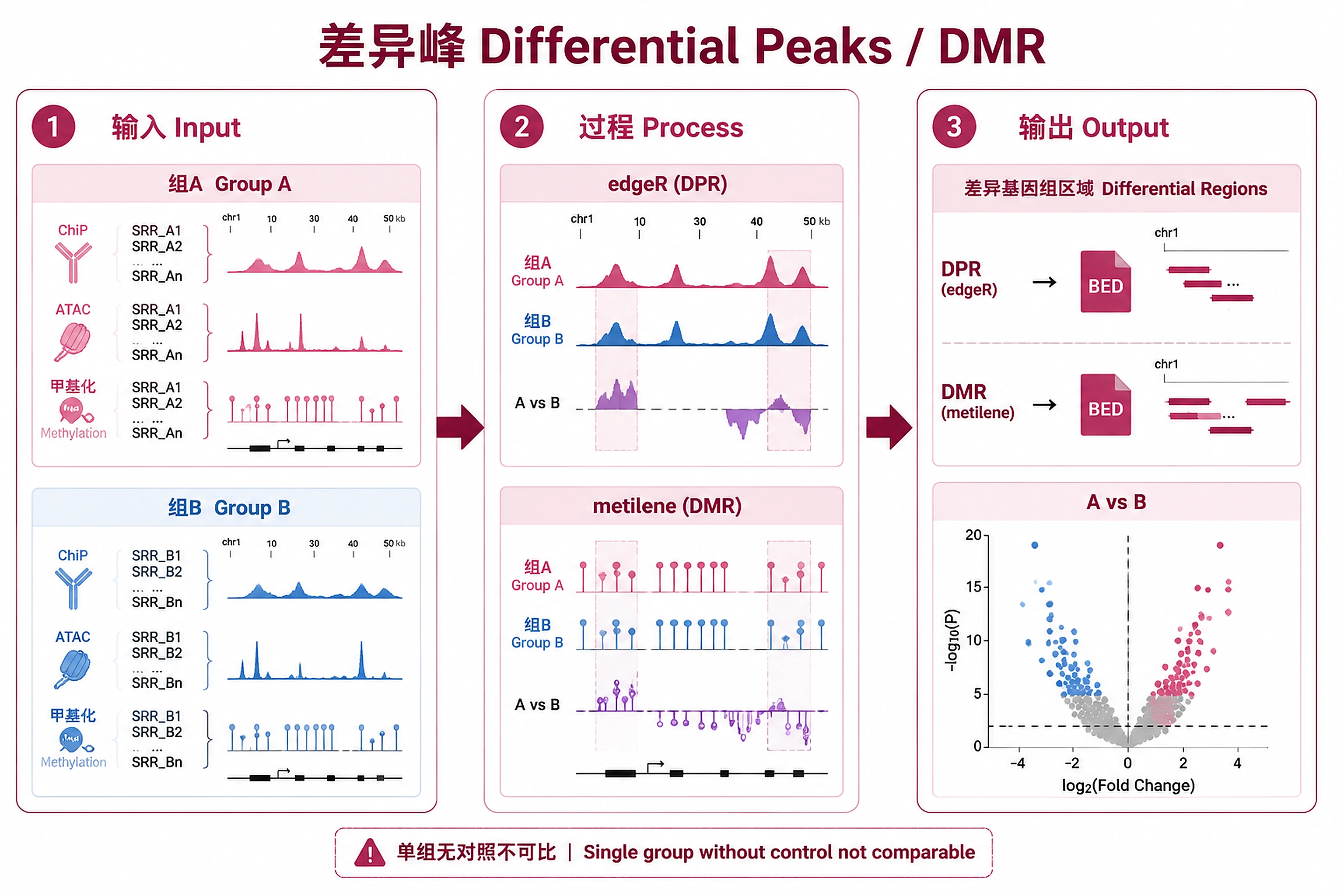
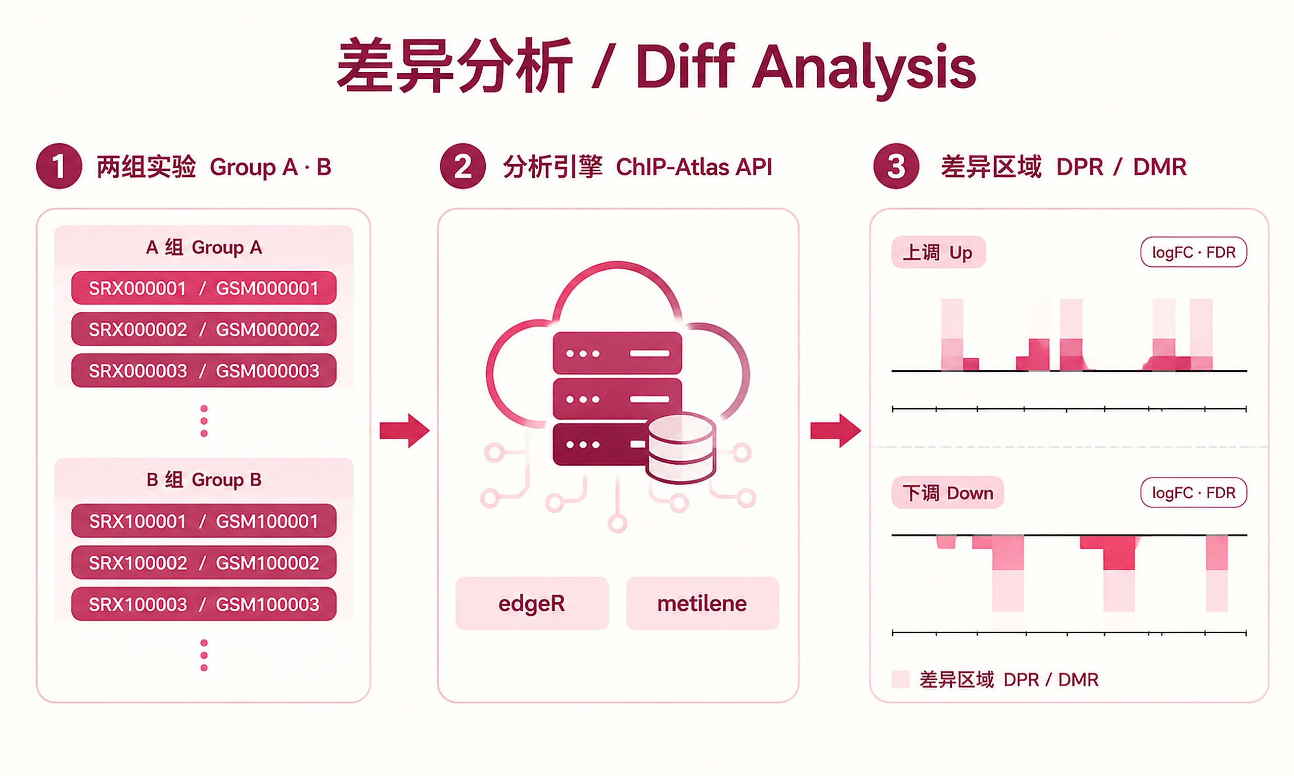
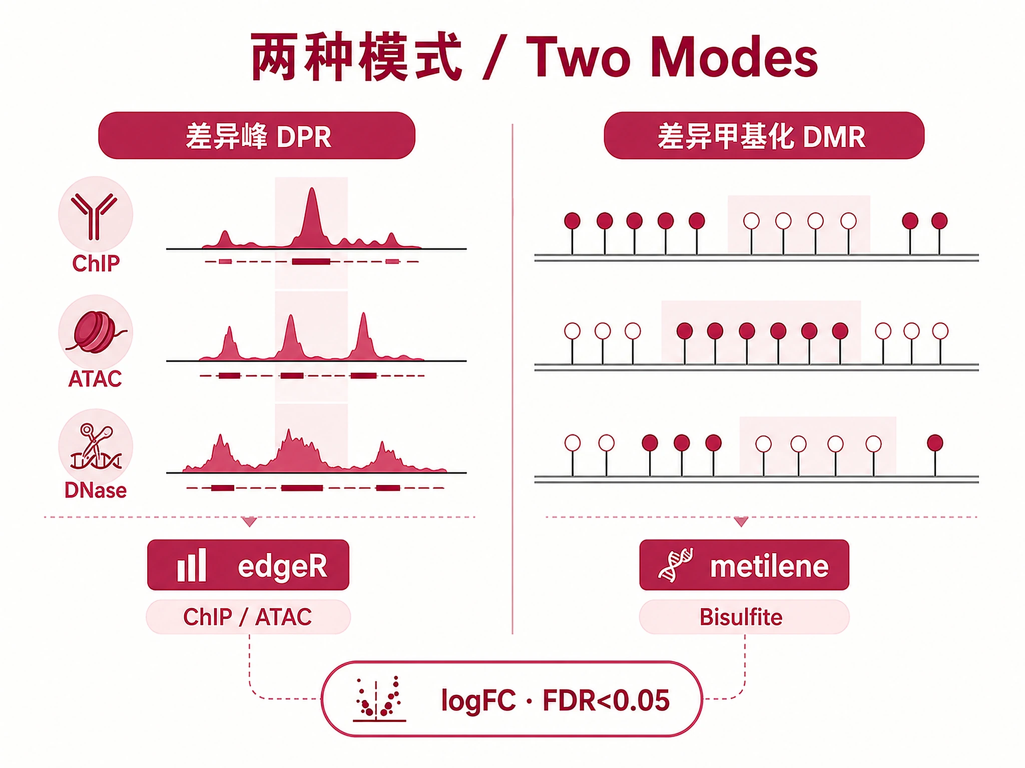
Compare two groups of experiments to identify differential peak regions (DPR) or differentially methylated regions (DMR) using the ChIP-Atlas Diff Analysis API.
When to Use This Skill
Use ChIP-Atlas diff analysis when you need to:
- Find differential peaks between two conditions (treated vs control, tissue A vs B)
- Identify differentially methylated regions between sample groups (Bisulfite-seq)
- Compare chromatin accessibility between cell types using ATAC-seq/DNase-seq data
- Leverage edgeR-based statistical framework on ChIP-Atlas public experiment data
- Avoid raw data downloads — works directly with experiment accession IDs
Don't use for:
- Single experiment analysis or peak calling (use MACS2/MACS3 workflows)
- Enrichment of factors near a gene list (use chip-atlas-peak-enrichment)
- Offline analysis (requires internet for API calls)
Key Concept: Submits two groups of experiment IDs to ChIP-Atlas. Server performs edgeR differential analysis (for DPR) or metilene (for DMR), returning BED files with genomic coordinates, logFC, p-values, q-values (FDR), and per-experiment normalized counts.
Installation
| Software | Version | License | Commercial Use | Installation |
|---|---|---|---|---|
| pandas | >=1.3 | BSD-3-Clause | Permitted | pip install pandas |
| requests | >=2.25 | Apache-2.0 | Permitted | pip install requests |
| numpy | >=1.20 | BSD-3-Clause | Permitted | pip install numpy |
| plotnine | >=0.10 | MIT | Permitted | pip install plotnine |
| plotnine-prism | >=0.2 | MIT | Permitted | pip install plotnine-prism |
pip install pandas requests numpy plotnine plotnine-prism
System requirements: Internet connection (API calls to ChIP-Atlas)
Inputs
Experiment IDs (two groups, minimum 2 per group):
- SRA accessions: SRX, ERX, DRX (e.g., SRX18419259)
- GEO accessions: GSM (e.g., GSM6765200)
- Formats: Python list, plain text (one per line), CSV with ID column
Parameters:
- Genome: hg38 (default), hg19, mm10, mm9, rn6, dm6, dm3, ce11, ce10, sacCer3
- Analysis type: "diffbind" (default, DPR for ChIP/ATAC/DNase-seq) or "dmr" (DMR for Bisulfite-seq)
Outputs
Analysis objects (Pickle):
analysis_object.pkl- Complete results for downstream use- Load with:
import pickle; obj = pickle.load(open('analysis_object.pkl', 'rb')) - Contains: diff_regions, diff_regions_unfiltered, qc_warnings, experiments_a/b, raw_files, log_content, parameters
Results (CSV):
diff_regions_all.csv- All differential regions, QC-filtered (chrom, start, end, logFC, pvalue, qvalue, direction, counts)diff_regions_significant.csv- Significant regions (FDR < 0.05)diff_regions_top50.csv- Top 50 by significance (with nearest gene annotation when available)diff_regions_unfiltered.csv- Pre-QC regions (includes non-standard contigs and regions < 10bp)
Raw results:
raw_results/- Original BED, IGV session, and log files from ChIP-Atlas
Visualizations (PNG + SVG, plotnine with Prism theme):
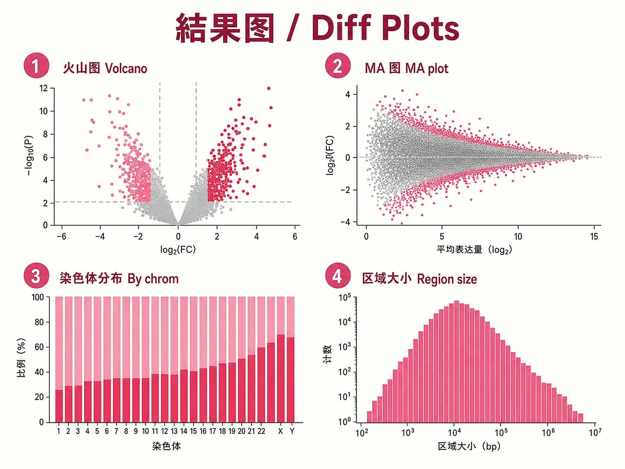
volcano_plot.png/.svg- Volcano plot (logFC vs -log10 Q-value)chromosome_distribution.png/.svg- Differential regions by chromosome (stacked bar)region_size_distribution.png/.svg- Region size histogram (log-scale)ma_plot.png/.svg- MA plot (mean counts vs logFC)
Reports:
summary_report.md- Human-readable analysis summary with QC warnings, nearest gene annotations, and statistical caveats
Clarification Questions
-
Input Files (ASK THIS FIRST):
- Do you have experiment IDs (SRX/GSM) for two groups to compare?
- Expected: At least 2 IDs per group (3+ recommended for statistical power)
- Formats: Plain text (one ID per line), CSV with ID column, or Python list
- Or use example data?
tp53_k562_dmso_vs_daunorubicin(recommended: TP53 K-562 DMSO vs Daunorubicin, n=8 vs n=8) ortp53_molm13_vs_k562(MOLM-13 vs K-562, n=4 vs n=4, demonstrates sex-chr QC)
-
Analysis parameters:
- Species/genome? Human hg38 (default), hg19, mouse mm10/mm9, rat rn6, fly, worm, yeast
- Analysis type? "diffbind" (default, for ChIP/ATAC/DNase-seq) or "dmr" (for Bisulfite-seq)
- Group labels? Names for each group (e.g., "Treated" vs "Control"). (Auto-set for example data.)
Standard Workflow
🚨 MANDATORY: USE SCRIPTS EXACTLY AS SHOWN - DO NOT WRITE INLINE CODE 🚨
Step 1 - Load data:
# Option 1: Example data
from scripts.load_example_data import load_example_data
data = load_example_data("tp53_k562_dmso_vs_daunorubicin")
experiments_a = data['experiments_a']
experiments_b = data['experiments_b']

# Option 2: Your own experiment IDs
# from scripts.load_user_data import load_user_data
# experiments_a = load_user_data("group_a.txt")
# experiments_b = load_user_data("group_b.txt")
✅ VERIFICATION: "✓ Data loaded successfully"
Step 2 - Run diff analysis:
from scripts.run_diff_workflow import run_diff_workflow

results = run_diff_workflow(
    experiments_a=experiments_a,
    experiments_b=experiments_b,
    genome=data.get('genome', 'hg38'),
    analysis_type=data.get('analysis_type', 'diffbind'),
    description_a=data.get('description_a', 'group_A'),
    description_b=data.get('description_b', 'group_B'),
    output_dir="diff_analysis_results"
)
DO NOT write inline API query code. Just use the script.
✅ VERIFICATION: "✓ Diff analysis completed successfully!"
Step 3 - Generate visualizations:
from scripts.generate_all_plots import generate_all_plots
generate_all_plots(results, output_dir="diff_analysis_results")
DO NOT write inline plotting code. The script handles PNG + SVG with graceful fallback.
✅ VERIFICATION: "✓ All visualizations generated successfully!"
Step 4 - Export results:
from scripts.export_all import export_all
export_all(results, output_dir="diff_analysis_results")
DO NOT write custom export code. Use export_all().
✅ VERIFICATION: "=== Export Complete ==="
⚠️ IF SCRIPTS FAIL - Hierarchy:
- Fix and Retry (90%) - Install missing package, check internet, re-run
- Modify Script (5%) - Edit the script, document changes
- Use as Reference (4%) - Read script, adapt approach
- Write from Scratch (1%) - Only if impossible, explain why
Common Issues
| Error | Cause | Solution |
|---|---|---|
| API 400 error | Invalid parameters | Check experiment IDs are valid (SRX/ERX/DRX/GSM format). See references/chipatlas_diff_api_format.md. |
| API timeout (>15 min) | Large dataset or server load | Normal for many experiments. Default timeout is 15 min. Reduce experiments per group if needed. |
| No BED file in ZIP | Analysis produced no results | Check experiment IDs exist in ChIP-Atlas. Ensure both groups have valid data for the selected genome. |
| Empty differential regions | No significant differences | Groups may be too similar. Try experiments from more distinct conditions. |
| requestId parse error | API response format changed | Check ChIP-Atlas server status. The API uses text format (not JSON) for diff analysis. |
| SVG export error | Missing optional dependency | Normal - generate_all_plots() handles fallback automatically. PNG always created. |
| chrY/chrX regions all one-directional | Sex chromosome confound | Groups differ in sex (male vs female cell lines). QC check flags this automatically. Exclude sex chromosome regions from biological interpretation. |
| Gene annotations missing | UCSC API unavailable | Normal in offline environments. Gene annotations are optional — all statistical results remain complete. |
Interpretation Guidelines
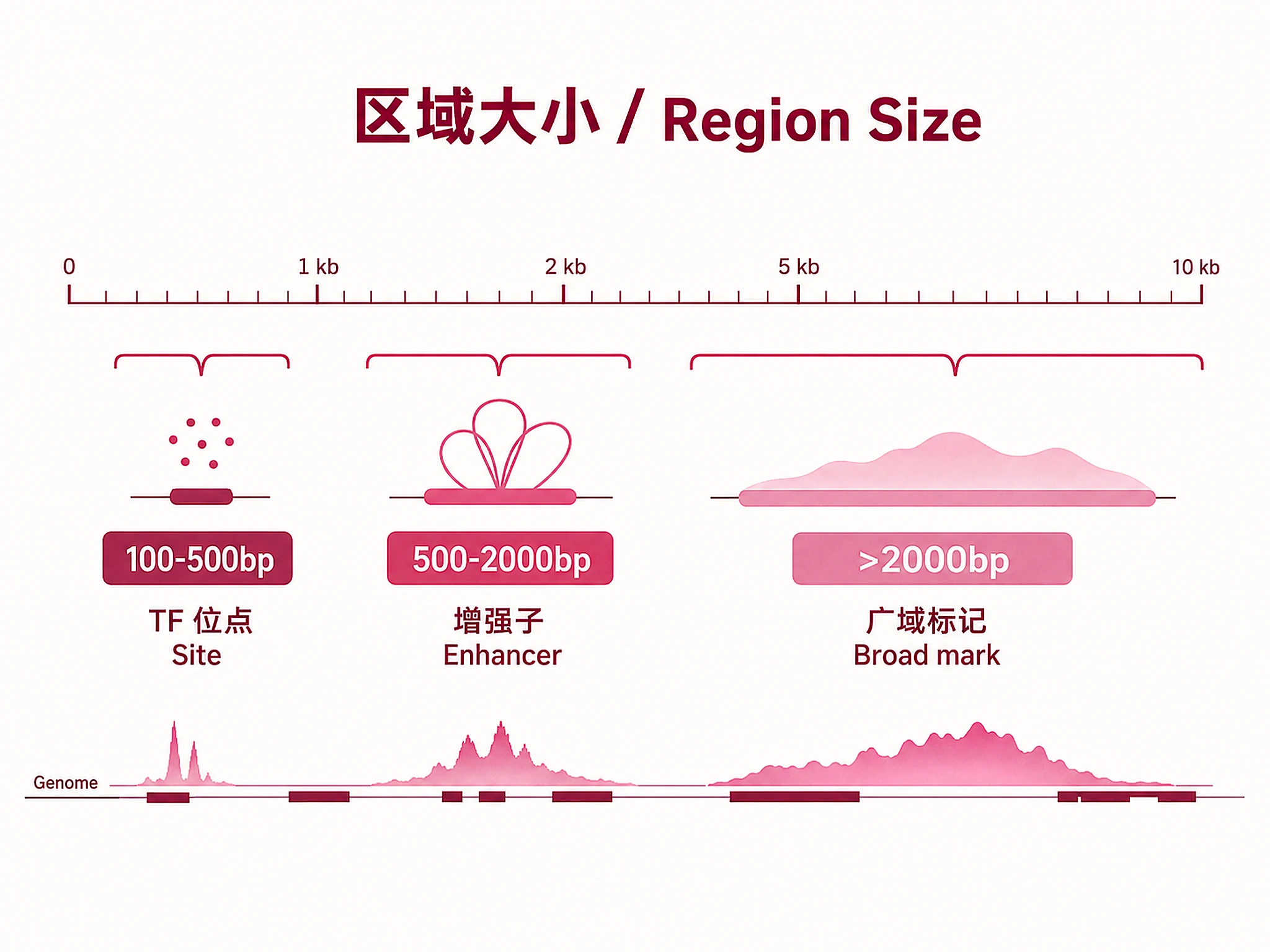
logFC: Log2 fold change — positive = enriched in Group A, negative = enriched in Group B Q-value (FDR): Benjamini-Hochberg corrected p-value — regions with FDR < 0.05 are significant Counts: TMM-normalized read counts per experiment (comma-separated in raw BED) Region Size: 100-500bp (TF sites), 500-2000bp (enhancers), >2000bp (broad marks)
Nearest gene annotations: Top regions in the summary report and top50 CSV are annotated with overlapping or nearby genes via UCSC REST API. Shows "GENE" for direct overlap or "GENE (+2.1kb)" for nearest gene within 5kb. Annotation is optional and skipped gracefully if the UCSC API is unavailable.
Automated QC checks (run automatically after Step 2):
- Sex chromosome confounds: If chrY/chrX regions are overwhelmingly one-directional with near-zero counts in the depleted group, this signals a sex mismatch between groups (e.g., male vs female cell lines). Checks both all regions (>80% threshold) and significant regions specifically (>67% threshold) to catch cases where noisy non-significant regions mask the artifact. These peaks should NOT be interpreted as genuine differential binding.
- Non-standard contigs: Regions on random scaffolds or unplaced sequences are filtered by default (mapping artifacts). Unfiltered data available in
diff_regions_unfiltered.csv. - Implausibly small regions: Regions < 10bp are filtered by default (edge artifacts — TF motifs are ~20bp, histone marks 200bp+).
- Genomic clusters: Dense clusters of one-directional significant regions (e.g., 10+ in <2 Mb) may indicate copy number amplification or structural variants rather than genuine differential binding. Investigate flagged clusters in a genome browser.
- chrM enrichment (ChIP-seq/ATAC-seq only): Mitochondrial DNA lacks histones and canonical chromatin structure. Significant differential regions on chrM in ChIP-seq or ATAC-seq experiments almost always reflect mitochondrial DNA contamination or non-specific antibody binding, not genuine transcription factor binding. Regions on chrM that are also <20bp are doubly suspect (too small for a TF binding site). chrM regions are NOT flagged for Bisulfite-seq (DMR mode), where mitochondrial methylation differences can be biologically meaningful.
- Sample size: With n ≤ 3, edgeR FDR values are unreliable — treat as approximate rankings. With n < 5, FDR estimates may be unstable. Focus on large effect sizes and validate key findings.
- MA plot asymmetry: If significant hits in one direction cluster at substantially lower mean counts than the other direction (>1 log2 unit difference in median), this may indicate normalization artifacts or noise-driven signal. Focus biological interpretation on higher-count significant regions.
- Unusually small regions: If the median significant region size is < 100bp for ChIP-seq/ATAC-seq, peak fragmentation may be inflating region counts. Check representative regions in a genome browser.
Reporting top hits: When summarizing top differential regions, present them in strict Q-value ranking order without skipping unannotated regions. Regions lacking gene annotations are still statistically significant. If you curate a subset (e.g., only gene-annotated hits), explicitly label the table as "selected highlights" — never imply it is a strict significance ranking. Accuracy: When quoting specific statistics (logFC, Q-values, coordinates) in your summary, copy values directly from summary_report.md or the CSV files — do NOT re-derive, round, or paraphrase numerical values from memory, as this introduces transcription errors.
Gene annotations: Nearest gene annotations indicate genomic proximity, not functional regulation. Describe associations factually (e.g., "a differential region near PCNA") without asserting direct regulatory relationships. Do not use individual gene annotations as validation of the analysis — gene proximity does not prove functional regulation.
Experimental design: edgeR treats all experiments within a group as biological replicates. If experiments within a group differ in important ways (e.g., different genotypes, tissues, or treatments), state this clearly — the differential analysis captures the average effect between groups, and within-group heterogeneity is treated as noise. When summarizing results to the user, design caveats MUST be stated prominently — not buried at the end. If within-group experiments are not true biological replicates, this is the single most important limitation to communicate.
MA plot interpretation: The MA plot shows mean expression (average log2 counts, x-axis) vs log fold change (y-axis). Normal pattern: funnel/fan shape narrowing at high counts (more power to detect small changes). Red flags: asymmetric significant hits clustering at low counts in one direction (potential normalization artifact), horizontal bands of significant hits (batch effects), or all significant hits at very low counts (noise-driven). CRITICAL: Do NOT claim MA plot asymmetry in your summary unless the automated QC check flagged it. The quantitative threshold is >1 log2 unit difference in median mean count between directions. Visual impressions of asymmetry below this threshold are not meaningful — small differences (e.g., 0.2 log2 units) are negligible and do not support claims of noise-driven signal. If no MA asymmetry QC warning appears, describe the MA plot as showing a normal pattern.
Biological interpretation of top hits: When discussing top differential regions near known genes, briefly note the gene's known function for context but do NOT claim the differential peak proves direct regulation. Genomic proximity does not establish causation. For exploratory analyses, suggest formal pathway/GO enrichment analysis as a next step to identify systematic patterns. Distinguish between confirmatory hits (regions near genes expected to differ) and exploratory hits (unexpected associations requiring validation). When the target factor is well-characterized (e.g., TP53, CTCF, ESR1, NF-kB), note whether canonical target genes appear in the top differential regions — the absence of expected targets is itself a notable finding that may indicate the differential signal is dominated by artifacts or indirect effects. After excluding artifact regions, comment on the effect sizes (logFC) of remaining biologically interpretable hits — modest effect sizes (|logFC| < 1.5) combined with annotations near pseudogenes or lncRNAs suggest limited genuine differential binding.
Citations: When writing your final summary, cite the data source (e.g., GSE accession) and key tools: ChIP-Atlas (Zou et al. 2024), edgeR (Robinson et al. 2010) for DPR, or metilene (Jühling et al. 2016) for DMR. Full references are in the References section below.
Caveats: Results depend on available public data quality. Always check QC warnings in the summary report. Validate key regions with orthogonal methods. See references/output_format.md for detailed output format.
Suggested Next Steps
- Visualize in IGV using the
.igv.xmlsession file or.igv.bedfile - Annotate regions with nearby genes using bedtools or GREAT
- Motif analysis on differential peaks (HOMER, MEME-ChIP)
- Integrate with expression data to link peaks to gene regulation
Related Skills
- chip-atlas-peak-enrichment - Enrichment of ChIP-seq peaks near gene lists
- bulk-rnaseq-counts-to-de-deseq2 - Differential expression to identify genes for downstream analysis
References
- Zou et al. (2024). ChIP-Atlas 3.0: a data-mining suite to explore chromosome architecture. Nucleic Acids Research. doi:10.1093/nar/gkad884
- Zou et al. (2022). ChIP-Atlas 2021 update. Nucleic Acids Research. doi:10.1093/nar/gkab933
- Robinson et al. (2010). edgeR: a Bioconductor package for differential expression analysis. Bioinformatics 26(1):139-140.
- Jühling et al. (2016). metilene: fast and sensitive calling of differentially methylated regions. Genome Research 26(2):256-262.
- ChIP-Atlas: https://chip-atlas.org
- API documentation: See references/chipatlas_diff_api_format.md
- Statistical methods: See references/diff_analysis_methods.md
Code preview
scripts/__init__.py
# chip-atlas-diff-analysis scripts packagescripts/annotate_genes.py
"""
Annotate differential regions with nearest/overlapping genes via UCSC REST API.

Uses the UCSC Genome Browser REST API to find genes overlapping or near
each genomic region. Requires internet (same as ChIP-Atlas API dependency).

Graceful fallback: if UCSC API is unavailable, returns empty annotations
without raising errors.
"""

import pandas as pd
import requests

UCSC_API_URL = "https://api.genome.ucsc.edu/getData/track"
FLANK_BP = 5000


def annotate_nearest_genes(df, genome="hg38", max_regions=50):
    """
    Annotate regions with overlapping/nearest gene symbols via UCSC API.

    Parameters
    ----------
    df : pd.DataFrame
        DataFrame with chrom, chromStart, chromEnd columns.
        Should be pre-sorted by significance (top regions first).
    genome : str
        UCSC genome assembly (hg38, mm10, etc.)
    max_regions : int
        Maximum number of regions to annotate (default: 50).

    Returns
    -------
    pd.Series
        Gene annotations indexed to match df. Each entry is a string
        like "SBF2" (overlapping) or "SBF2 (+2.1kb)" (nearest within flank).
        Empty string for unannotated regions.
    """
    annotations = pd.Series("", index=df.index)

    regions_to_query = df.head(max_regions)
    if len(regions_to_query) == 0:
        return annotations

    print(f"   Annotating top {len(regions_to_query)} regions with nearest genes (UCSC API)...")

    n_annotated = 0
    n_failed = 0

    for idx, row in regions_to_query.iterrows():
        try:
            gene_str = _query_genes_for_region(
                row["chrom"],
                int(row["chromStart"]),
                int(row["chromEnd"]),
                genome=genome,
            )
            if gene_str:
                annotations.at[idx] = gene_str
                n_annotated += 1
        except Exception:
            n_failed += 1
            if n_failed >= 3:
                print(f"   Warning: UCSC API unavailable ({n_failed} failures). "
                      f"Skipping remaining gene annotations.")
                break

    print(f"   Annotated {n_annotated}/{len(regions_to_query)} regions with gene symbols")
    return annotations


def _query_genes_for_region(chrom, start, end, genome="hg38"):
    """
    Query UCSC REST API for genes overlapping or near a region.

    Returns
    -------
    str
        Gene symbol(s) or empty string.
        Direct overlap: "GENE1, GENE2"
scripts/export_all.py
"""
Export all ChIP-Atlas diff analysis results (Step 4).

Exports:
1. analysis_object.pkl - Complete results for downstream use
2. diff_regions_all.csv - All differential regions
3. diff_regions_significant.csv - Significant regions (FDR < 0.05)
4. diff_regions_top50.csv - Top 50 by significance
5. summary_report.md - Human-readable summary
"""

import os
import pickle
from datetime import datetime

try:
    try:
        from scripts.annotate_genes import annotate_nearest_genes
    except ImportError:
        from annotate_genes import annotate_nearest_genes
    _HAS_GENE_ANNOTATION = True
except ImportError:
    _HAS_GENE_ANNOTATION = False


def export_all(results, output_dir="diff_analysis_results", qvalue_threshold=0.05):
    """
    Export all ChIP-Atlas diff analysis results with pickle object.

    Parameters
    ----------
    results : dict
        Results from run_diff_workflow()
    output_dir : str
        Output directory
    qvalue_threshold : float
        Maximum Q-value (FDR) for "significant" regions (default: 0.05)

    Verification
    ------------
    Prints "=== Export Complete ===" when done
    """
    os.makedirs(output_dir, exist_ok=True)

    print("\n" + "=" * 70)
    print("EXPORTING RESULTS")
    print("=" * 70 + "\n")

    df = results["diff_regions"]
    params = results["parameters"]

    qc_warnings = results.get("qc_warnings", [])
    unfiltered_df = results.get("diff_regions_unfiltered", df)

    # 1. Save analysis object as pickle (CRITICAL for downstream skills)
    print("1. Saving analysis objects for downstream use...")

    n_a = (df["direction"] == "A_enriched").sum() if len(df) > 0 else 0
    n_b = (df["direction"] == "B_enriched").sum() if len(df) > 0 else 0

    analysis_object = {
        "diff_regions": df,
        "diff_regions_unfiltered": unfiltered_df,
        "qc_warnings": qc_warnings,
        "experiments_a": results["experiments_a"],
        "experiments_b": results["experiments_b"],
        "raw_files": results.get("raw_files", {}),
        "log_content": results.get("log_content", ""),
        "parameters": params,
        "n_regions_total": len(df),
        "n_regions_unfiltered": len(unfiltered_df),
        "n_regions_a_enriched": int(n_a),
        "n_regions_b_enriched": int(n_b),
        "timestamp": datetime.now().isoformat(),
    }

    pickle_path = os.path.join(output_dir, "analysis_object.pkl")
    with open(pickle_path, "wb") as f:
        pickle.dump(analysis_object, f)
Companion files
| Type | Path | Bytes |
|---|---|---|
| Markdown | references/chipatlas_diff_api_format.md | 3,114 |
| Markdown | references/diff_analysis_methods.md | 3,082 |
| Markdown | references/output_format.md | 2,955 |
| Python | scripts/__init__.py | 43 |
| Python | scripts/annotate_genes.py | 4,346 |
| Python | scripts/export_all.py | 23,617 |
| Python | scripts/filter_regions.py | 5,816 |
| Python | scripts/generate_all_plots.py | 10,544 |
| Python | scripts/load_example_data.py | 6,108 |
| Python | scripts/load_user_data.py | 6,774 |
| Python | scripts/parse_bed_results.py | 8,029 |
| Python | scripts/qc_checks.py | 23,954 |
| Python | scripts/query_chipatlas_api.py | 10,536 |
| Python | scripts/run_diff_workflow.py | 8,941 |
| Markdown | SKILL.md | 16,221 |
| JSON | skill.meta.json | 3,044 |