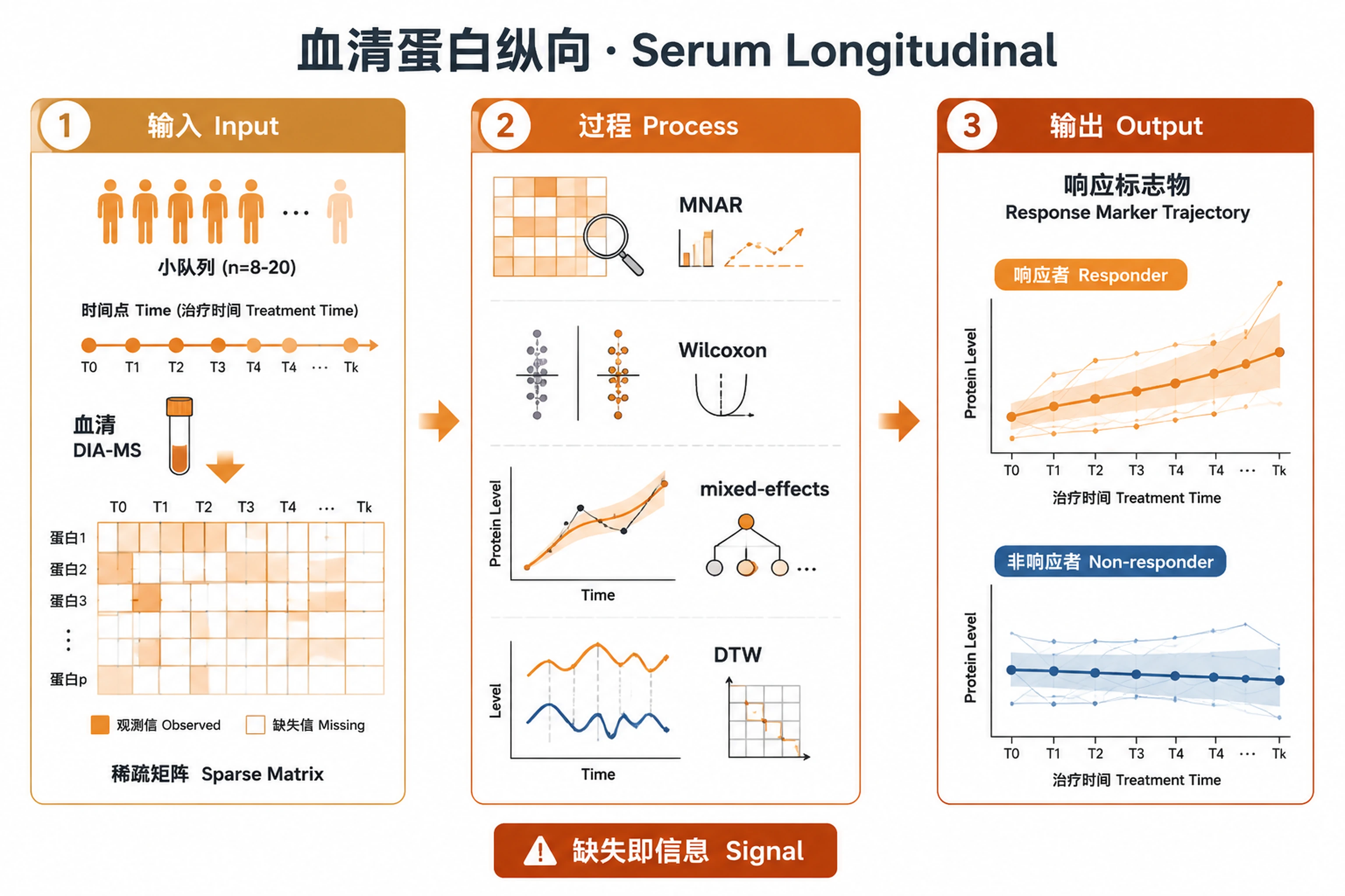
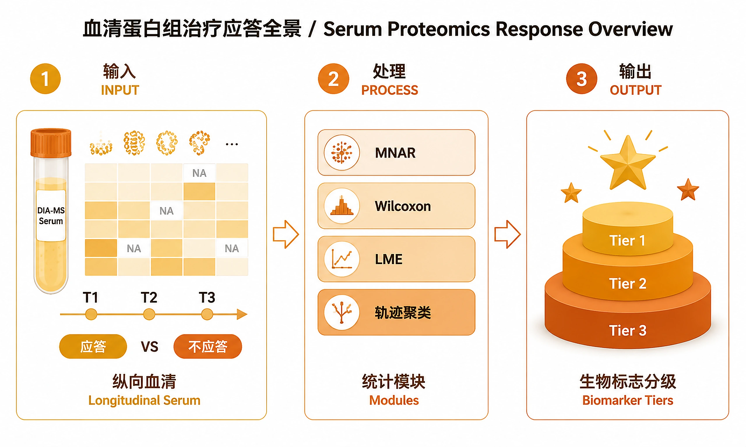
Serum Proteomics, Longitudinal
A full DIA-MS pipeline for longitudinal treatment response.
Overview
Problem. Find response markers in small, sparse, longitudinal data.
Learning goals
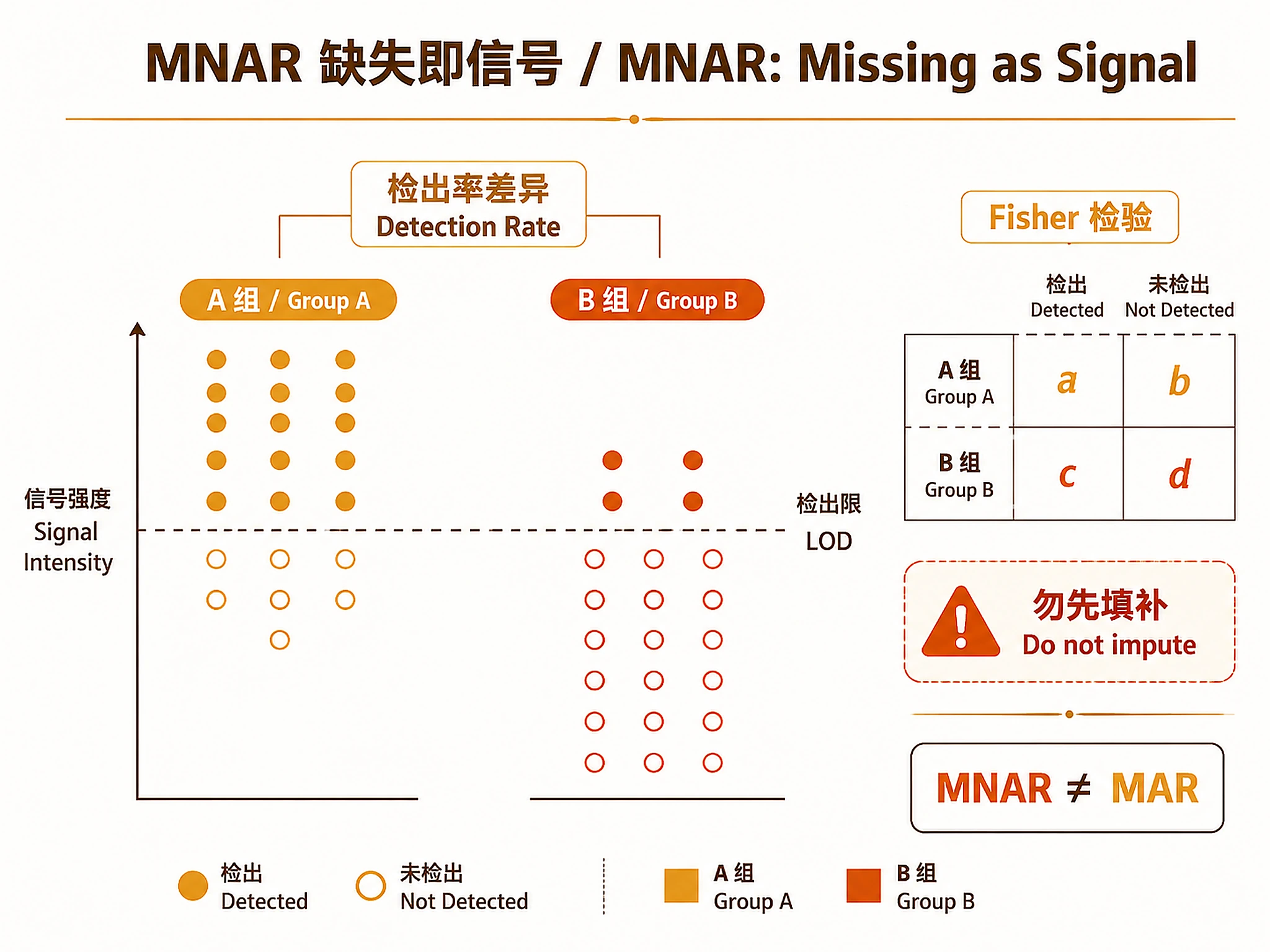
- Missingness itself can be signal (MNAR)
- Non-parametric for small n; mixed models for longitudinal
Figures

Tutorial
When to Use This Skill
Use this skill when ALL of the following are true:
- You have serum or plasma proteomics data (DIA-MS, Olink, SomaScan, or similar)
- The study has ≥2 longitudinal timepoints (e.g., baseline T1, mid-treatment T2, end T3)
- Samples are from ≥2 response groups (e.g., Early Responder, Poor Responder)
- You want MNAR detection, longitudinal modelling, or biomarker tiering — not just standard DE
Do NOT use this skill for:
- TMT/LFQ proteomics with PSM counts → use
proteomics-diff-exp(limma + DEqMS) - LASSO panel with nested cross-validation → use
lasso-biomarker-panel - Pathway enrichment of DE proteins → use
functional-enrichment-from-degs - Single-timepoint case-control proteomics without MNAR concern → use
proteomics-diff-exp
Inputs
| Input | Format | Required |
|---|---|---|
| Protein intensity matrix | CSV: rows = protein names, cols = sample IDs; NA = not detected (below LOD) |
Required |
| Sample metadata | CSV: sample_id, patient_id, timepoint (T1/T2/T3), response_group + optional covariates |
Required |
| Clinical score table | CSV: patient_id, timepoint, PASI (or equivalent score) |
Optional — enables trajectory clustering |
| Cross-species DE table | CSV: protein, log2FC, p_value, direction (from mouse model) |
Optional — enables cross-species tier bonus |
Input format notes
- Intensity values: Log2-transformed preferred. If raw intensities (median > 100), scripts auto-apply log2.
- NA encoding: Use
NAor empty cells for non-detected proteins. Do NOT use 0 — zero is a valid intensity. - Sample IDs: Must match between intensity matrix column names and metadata
sample_idcolumn. - Protein names: Use gene symbols (CHGA, SCG2, ITIH1) or UniProt accessions. Consistent naming required.
- Supported platforms: Spectronaut 16 (DIA-MS), MaxQuant (LFQ), Olink NPX, SomaScan RFU — any platform that produces a protein × sample matrix with NA for non-detection.
Outputs
| File | Description |
|---|---|
results/mnar_results.csv |
Per-protein MNAR classification: detection rates by group, Fisher p, Fisher adj_p, MNAR direction |
results/de_results.csv |
Full DE table: log2FC, Wilcoxon p, BH adj_p, MNAR flag, direction |
results/de_results_significant.csv |
Significant DE proteins only (adj_p < threshold OR MNAR) |
results/lme_results.csv |
Per-protein LME: time×group interaction p, adj_p, trajectory type, T2 coefficient |
results/trajectory_clusters.csv |
Patient-level cluster assignments, cluster label, Flare→Clear flag |
results/biomarker_tiers.csv |
Primary output: Tier 1/2/3 ranking with MNAR flag, LME interaction p, cross-species flag, mechanistic annotation |
results/biomarker_tier1_priority.csv |
Tier 1 proteins only — immediate ELISA validation candidates |
results/analysis_object.rds |
Complete pipeline object for downstream skills |
results/analysis_summary.txt |
Plain-text summary of all modules |
Installation
options(repos = c(CRAN = "https://cloud.r-project.org"))

# Core (required)
install.packages(c("dplyr", "tidyr", "nlme"))

# Trajectory clustering (strongly recommended)
install.packages(c("dtw", "cluster"))

# Downstream skills
if (!require("BiocManager", quietly = TRUE)) install.packages("BiocManager")
BiocManager::install("limma")   # for proteomics-diff-exp upstream
install.packages(c("glmnet", "pROC"))  # for lasso-biomarker-panel downstream
| Package | Version | Purpose |
|---|---|---|
| dplyr | ≥1.1 | Data manipulation |
| tidyr | ≥1.3 | Pivoting |
| nlme | ≥3.1 | Mixed-effects models |
| dtw | ≥1.22 | DTW distance for trajectory clustering |
| cluster | ≥2.1 | Silhouette width for optimal k |
Standard Workflow
MANDATORY: SOURCE SCRIPTS — DO NOT WRITE INLINE CODE
Step 0 — Load data
# Load your protein intensity matrix (rows = proteins, cols = samples, NA = not detected)
intensity_matrix <- read.csv("your_protein_matrix.csv", row.names = 1, check.names = FALSE)

# Load sample metadata
metadata <- read.csv("your_metadata.csv", stringsAsFactors = FALSE)
# Required columns: sample_id, patient_id, timepoint, response_group

# Optional: clinical score table for trajectory clustering
score_table <- read.csv("your_pasi_scores.csv", stringsAsFactors = FALSE)
# Required columns: patient_id, timepoint, PASI (or your score column)

# Optional: cross-species DE table
xspecies_df <- read.csv("your_mouse_de.csv", stringsAsFactors = FALSE)
# Required columns: protein, log2FC, p_value, direction
VERIFICATION: Check dimensions and NA pattern:
cat(sprintf("Matrix: %d proteins × %d samples\n", nrow(intensity_matrix), ncol(intensity_matrix)))
cat(sprintf("Missing values: %.1f%%\n", 100 * mean(is.na(intensity_matrix))))
cat(sprintf("Metadata: %d rows, groups: %s\n",
    nrow(metadata), paste(unique(metadata$response_group), collapse=", ")))
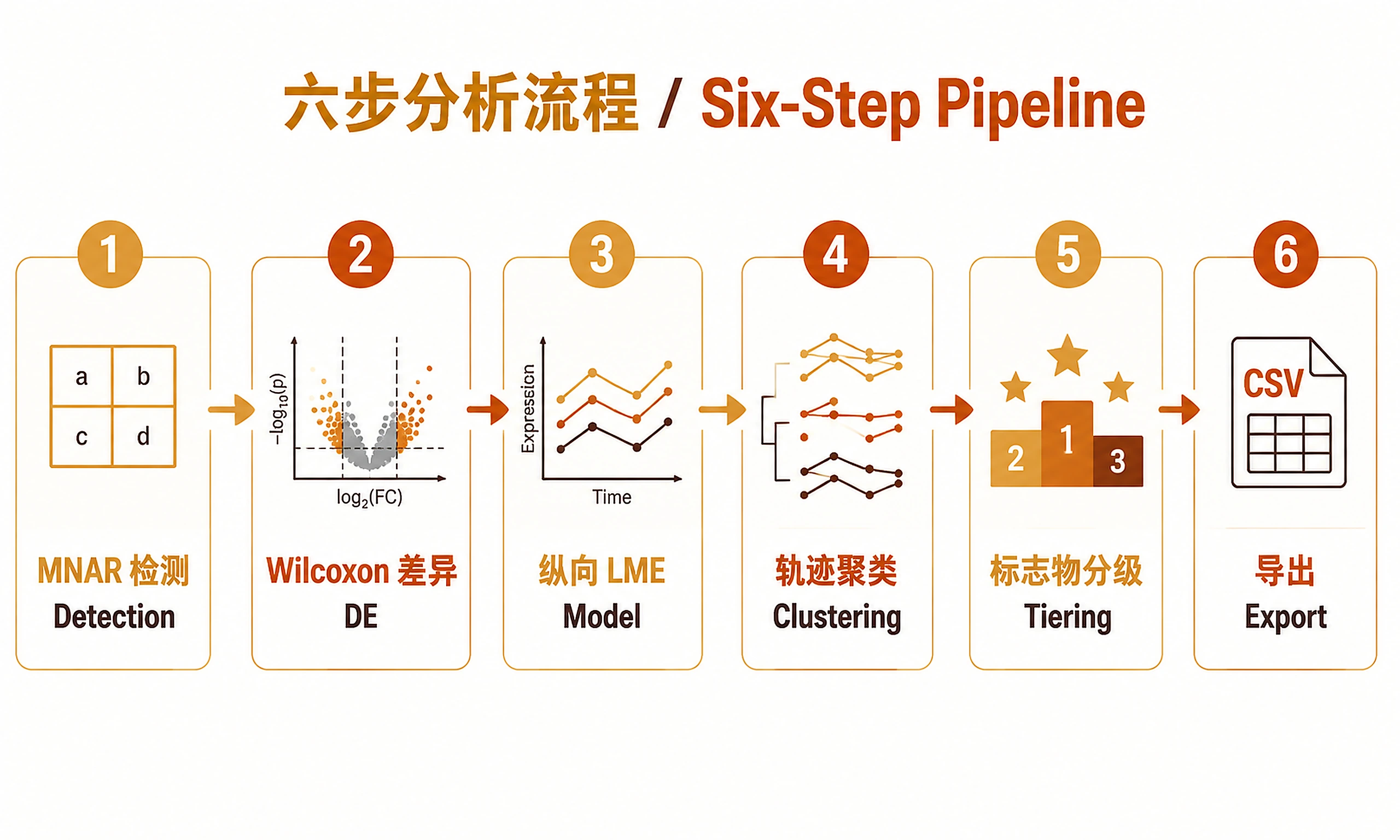
Step 1 — MNAR Detection
source("scripts/01_mnar_detection.R")

mnar_result <- run_mnar_detection(
  intensity_matrix = intensity_matrix,
  metadata         = metadata,
  params = list(
    baseline_timepoint = "T1",       # timepoint for MNAR test
    response_col       = "response_group",
    sample_col         = "sample_id",
    mnar_fisher_p      = 0.05        # Fisher p threshold
  )
)

# Optional: check granin dissociation pattern (CHGA vs SCG2)
check_granin_dissociation(mnar_result$mnar_table,
  params = list(responder_group = "Early"))
VERIFICATION: You MUST see "✓ MNAR detection complete." with a count of MNAR proteins.
DO NOT impute MNAR proteins before this step. Imputation destroys the MNAR signal.
Step 2 — Wilcoxon Differential Expression
source("scripts/02_wilcoxon_de.R")

de_result <- run_wilcoxon_de(
  intensity_matrix = intensity_matrix,
  metadata         = metadata,
  mnar_table       = mnar_result$mnar_table,   # pass MNAR flags
  params = list(
    de_timepoint      = "T1",          # baseline comparison
    response_col      = "response_group",
    sample_col        = "sample_id",
    group_a           = "Early",       # numerator group
    group_b           = "Poor",        # denominator group
    de_adj_p          = 0.05,
    de_log2fc         = 0.58,
    min_detected_frac = 0.5
  )
)

# Quick volcano summary (text)
summarise_volcano(de_result$de_table)
VERIFICATION: You MUST see "✓ Wilcoxon DE complete." with significant protein counts.
Note: MNAR proteins are automatically appended to the DE table with is_mnar = TRUE and wilcox_p = NA. They are included in the biomarker tiering step.
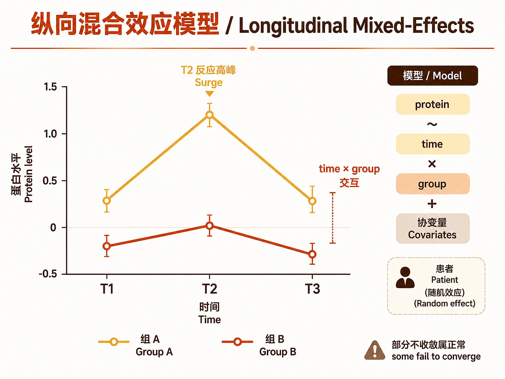
Step 3 — Longitudinal Mixed-Effects Modelling
source("scripts/03_longitudinal_lme.R")

lme_result <- run_longitudinal_lme(
  intensity_matrix = intensity_matrix,
  metadata         = metadata,
  params = list(
    timepoints        = c("T1", "T2", "T3"),
    timepoint_col     = "timepoint",
    response_col      = "response_group",
    patient_col       = "patient_id",
    covariates        = c("baseline_PASI", "age", "sex"),  # adjust to your metadata
    ref_timepoint     = "T1",
    ref_group         = "Poor",          # reference group for contrasts
    lme_interaction_p = 0.05,
    t2_surge_group    = "Early"          # group expected to show T2 surge
  )
)
VERIFICATION: You MUST see "✓ Longitudinal LME complete." with interaction counts.
Note on convergence: 5–15% of proteins may fail to converge — this is normal. They are flagged as model_status = "model_failed" and excluded from interaction ranking but retained in the DE table.
Skip this step if: You have only 1 timepoint, or fewer than 3 patients with repeated measures.
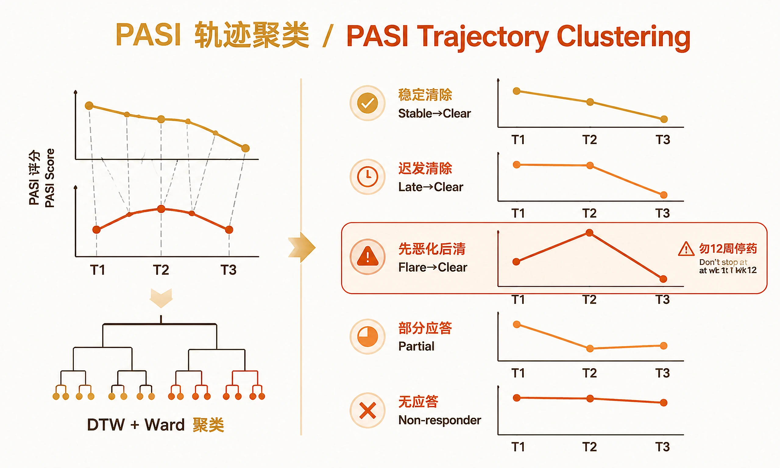
Step 4 — PASI Trajectory Clustering (Optional)
source("scripts/04_trajectory_clustering.R")

cluster_result <- run_trajectory_clustering(
  score_table = score_table,
  params = list(
    patient_col   = "patient_id",
    timepoint_col = "timepoint",
    score_col     = "PASI",
    timepoints    = c("T1", "T2", "T3"),   # NULL = auto-detect
    k_range       = 2:7,
    flare_ratio   = 1.2,    # T2/T1 > 1.2 = flare
    clear_ratio   = 0.5     # T3/T1 < 0.5 = PASI50 response
  )
)
VERIFICATION: You MUST see "✓ Trajectory clustering complete." with cluster summary table.
CRITICAL CLINICAL NOTE: If Flare→Clear patients are identified, do NOT recommend treatment discontinuation at 12 weeks based on T2 PASI alone. These patients show transient worsening before resolution — a pattern that would be misclassified as non-response under a standard 12-week endpoint.
Skip this step if: You have no clinical score data, or only 1 timepoint.
Step 5 — Biomarker Tiering
source("scripts/05_biomarker_tiering.R")

tier_result <- run_biomarker_tiering(
  de_result   = de_result,
  lme_result  = lme_result,    # NULL if Step 3 was skipped
  xspecies_df = xspecies_df,   # NULL if no cross-species data
  params = list(
    tier1_mnar_adj_p      = 0.001,
    tier1_lme_adj_p       = 0.001,
    tier1_require_t2surge = TRUE,
    tier2_de_adj_p        = 0.01,
    tier2_de_log2fc       = 1.0,
    tier3_de_adj_p        = 0.05,
    tier3_de_log2fc       = 0.58
  )
)
VERIFICATION: You MUST see "✓ Biomarker tiering complete." with Tier 1/2/3 counts.
Step 6 — Export All Results
source("scripts/06_export_results.R")

export_all(
  mnar_result    = mnar_result,
  de_result      = de_result,
  lme_result     = lme_result,       # NULL if skipped
  cluster_result = cluster_result,   # NULL if skipped
  tier_result    = tier_result,
  output_dir     = "results",
  study_label    = "MMIP_psoriasis"  # change to your study name
)
VERIFICATION: You MUST see "=== Export Complete ===" with file list.
Parameters Reference
| Parameter | Default | Description |
|---|---|---|
baseline_timepoint |
"T1" |
Timepoint used for MNAR test and baseline DE |
timepoints |
c("T1","T2","T3") |
All timepoints in longitudinal order |
response_col |
"response_group" |
Column name for responder classification |
patient_col |
"patient_id" |
Column for random effect (repeated measures) |
sample_col |
"sample_id" |
Column linking metadata to matrix columns |
score_col |
"PASI" |
Clinical score column for trajectory clustering |
group_a |
first group | Numerator group for log2FC (positive = higher in A) |
group_b |
second group | Denominator group for log2FC |
mnar_fisher_p |
0.05 |
Fisher p threshold for MNAR classification |
de_adj_p |
0.05 |
BH-adjusted p threshold for DE significance |
de_log2fc |
0.58 |
|log2FC| threshold (~1.5-fold) |
lme_interaction_p |
0.05 |
Time×group interaction adj_p threshold |
covariates |
c() |
Fixed-effect covariates in LME (must be in metadata) |
t2_surge_group |
NULL |
Group expected to show T2 surge (for trajectory classification) |
flare_ratio |
1.2 |
T2/T1 ratio threshold for "flare" classification |
clear_ratio |
0.5 |
T3/T1 ratio threshold for "clear" (PASI50 equivalent) |
tier1_mnar_adj_p |
0.001 |
Fisher adj_p threshold for Tier 1 MNAR |
tier1_lme_adj_p |
0.001 |
LME interaction adj_p threshold for Tier 1 |
tier2_de_adj_p |
0.01 |
DE adj_p threshold for Tier 2 |
tier2_de_log2fc |
1.0 |
|log2FC| threshold for Tier 2 (2-fold) |
Worked Example: MMIP Psoriasis Cohort
Study design: n=90 psoriasis patients, DIA-MS serum proteomics, 3 timepoints (T1=baseline, T2=12 weeks, T3=1 year), 3 response groups (Early Responder n=10, Late Responder n=10, Poor Responder n=10 for discovery; n=60 for validation).
Expected results from this pipeline:
| Module | Key finding |
|---|---|
| MNAR detection | CHGA: detected in 1/10 Early Responders vs 9/10 Poor Responders (Fisher p<0.001, FDR q=1.45×10⁻⁹) → Tier 1 |
| MNAR detection | SCG2: inverse pattern — detected in 8/10 Early Responders → granin dissociation |
| Wilcoxon DE | AGT, CBG, KLKB1, KNG1 elevated in Early Responders (adj_p<0.05) → Tier 2/3 |
| Wilcoxon DE | ITIH1 lower in Poor Responders at T1 (adj_p=0.049) → Tier 3 |
| LME | SAA1, DBI: significant time×group interaction (T2 surge in Early Responders) → Tier 1 |
| LME | ITIH1: progressive decline in Poor Responders (interaction p=0.049) → Tier 2 |
| Trajectory clustering | 5 clusters: Stable→Clear, Late→Clear, Flare→Clear, Partial, Non-responder |
| Trajectory clustering | Flare→Clear patients: T2 PASI worsening then 1yr resolution — do not discontinue |
| Biomarker tiering | Tier 1: CHGA (MNAR), SAA1 (T2 surge), DBI (T2 surge) |
| Biomarker tiering | Tier 2: ITIH1, AGT, CBG, KLKB1, KNG1, SCG2 |
| Biomarker panel | CHGA + ITIH1 AUC = 0.87 (95% CI 0.79–0.95) for Early vs Poor Responder |
Biological interpretation:
- CHGA MNAR in Early Responders = chromaffin granule depletion = "low-reserve" sympatho-adrenal state. These patients have already mobilised their catecholamine stores before treatment, making them primed to respond to psychological intervention.
- SAA1 T2 surge in Early Responders = acute-phase reactogenicity at 12 weeks = the immune system is actively responding to the psychological therapy. This is a marker of engagement, not failure.
- ITIH1 decline in Poor Responders = progressive ECM destabilisation = ongoing inflammation without resolution.
Clarification Questions
ALWAYS ask Question 1 FIRST.
1. Data availability
- Do you have a protein intensity matrix with NA values for non-detected proteins?
- If yes: proceed to Question 2
- If no (all proteins quantified, no NAs): MNAR step will find nothing — consider
proteomics-diff-expinstead
2. Study design
- How many timepoints? (2 = skip LME; 3+ = run full longitudinal model)
- How many patients per response group? (< 5 per group = results unreliable; 8–15 = typical discovery cohort)
- Do you have clinical score data (PASI or equivalent) for trajectory clustering?
3. Response group definition
- Are response groups pre-defined in your metadata, or do you need to derive them from clinical scores?
- Pre-defined: proceed directly
- Need to derive: use PASI50/75/90 thresholds or trajectory clustering first, then re-run DE
4. Covariates
- Which covariates are available in your metadata for the LME model?
- Recommended: baseline clinical score, age, sex
- If none available: run without covariates (set
covariates = c())
Common Issues
| Issue | Cause | Fix |
|---|---|---|
"No overlap between metadata sample_ids and intensity_matrix column names" |
Column name mismatch | Check colnames(intensity_matrix) vs metadata$sample_id — must be identical strings |
"No samples found for timepoint 'T1'" |
Wrong timepoint label | Check unique(metadata$timepoint) and set baseline_timepoint to match |
All proteins show mnar_class = "undetected_all" |
NA encoding issue | Ensure non-detected proteins are NA, not 0 or "" |
| LME convergence failures > 50% | Too few repeated measures | Check each patient has ≥2 timepoints; reduce covariates if overparameterised |
dtw package not found |
Not installed | install.packages("dtw") — falls back to Euclidean distance automatically |
cluster package not found |
Not installed | install.packages("cluster") — falls back to k=3 automatically |
| Tier 1 is empty | Thresholds too stringent | Relax tier1_mnar_adj_p to 0.01 or tier1_lme_adj_p to 0.01 |
| log2FC direction unexpected | group_a/group_b swapped | log2FC = median(group_a) - median(group_b); swap group_a and group_b |
"Need at least 4 patients for clustering" |
Too few patients | Trajectory clustering requires ≥4 patients; skip Step 4 for very small cohorts |
Interpretation Guidelines
MNAR results
MNAR_up_in_X: protein is MORE OFTEN detected in group X → group X has higher circulating levels (above LOD)MNAR_down_in_X: protein is LESS OFTEN detected in group X → group X has lower levels (below LOD)- CHGA MNAR in responders = responders have LOWER CHGA (below LOD) = chromaffin granule depletion
DE results
log2FC > 0= higher in group_a;log2FC < 0= higher in group_b- MNAR proteins have
wilcox_p = NA— their significance comes fromfisher_adj_p - Do NOT interpret MNAR proteins using log2FC alone
LME results
trajectory_type = "T2_surge"= protein rises at T2 specifically in the surge grouptrajectory_type = "T2_dip"= protein falls at T2 specifically in the surge groupmodel_status = "model_failed"= convergence failure — not a biological finding
Biomarker tiers
- Tier 1 (★★★): Recommend for immediate ELISA validation in independent cohort
- Tier 2 (★★): Recommend for multiplexed panel (Luminex/Olink) validation
- Tier 3 (★): Hypothesis-generating only; do not prioritise for validation without additional evidence
- Mechanistic annotation:
"unknown"is not a negative finding — it may indicate a novel axis
AUC / ROC
- AUC values reported in
analysis_summary.txtare from the discovery cohort only - These are expected to be optimistic; external validation is required before clinical claims
- For validated AUC, use
lasso-biomarker-panelwith an independent cohort
Suggested Next Steps
After running this skill:
- ELISA validation of Tier 1 proteins in independent cohort → use
biomarker_tier1_priority.csv - LASSO panel from Tier 1+2 proteins →
lasso-biomarker-panel(input:de_results_significant.csv) - Pathway enrichment of significant DE proteins →
functional-enrichment-from-degs - Mendelian randomisation for causal inference on top candidates →
mendelian-randomization-twosamplemr - Cross-species validation in mouse model (IMQ psoriasis) → re-run with mouse serum proteomics and pass as
xspecies_df
Related Skills
| Skill | Relationship | When to use |
|---|---|---|
proteomics-diff-exp |
Upstream | PSM aggregation, TMT/LFQ normalization before this skill |
lasso-biomarker-panel |
Downstream | Build minimal ELISA panel from Tier 1+2 proteins |
functional-enrichment-from-degs |
Downstream | Pathway enrichment of DE protein list |
mendelian-randomization-twosamplemr |
Downstream | Causal inference for top biomarker candidates |
disease-progression-longitudinal |
Alternative | Pseudotime-based trajectory inference (single-cell) |
survival-analysis-clinical |
Downstream | Time-to-response analysis using biomarker tiers |
References
- MNAR handling: Lazar C, et al. (2016) J Proteome Res 15(4):1116–1125
- Wilcoxon for small proteomics: Kammers K, et al. (2015) EuPA Open Proteomics 7:11–19
- nlme mixed-effects: Pinheiro J, Bates D (2000) Mixed-Effects Models in S and S-PLUS. Springer
- DTW clustering: Sakoe H, Chiba S (1978) IEEE Trans Acoust 26(1):43–49
- BH correction: Benjamini Y, Hochberg Y (1995) J R Stat Soc B 57(1):289–300
- MMIP study: Wan F, et al. (in preparation) — Sympatho-adrenal hypothesis for psoriasis treatment response
- See references/method-notes.md for full statistical rationale
Code preview
scripts/01_mnar_detection.R
# =============================================================================
# 01_mnar_detection.R
# Missing-Not-At-Random (MNAR) protein detection for serum proteomics
#
# Purpose:
#   Identify proteins whose absence from serum is non-random with respect to
#   treatment response group. In DIA-MS data, a protein below the detection
#   limit (NA) carries biological information distinct from a low-abundance
#   quantified protein. This script separates MNAR proteins from quantified
#   proteins before downstream DE analysis.
#
# Inputs (loaded from environment or passed as arguments):
#   intensity_matrix  - data.frame, rows = proteins, cols = sample_ids
#                       NA values indicate non-detection (below LOD)
#   metadata          - data.frame with columns: sample_id, patient_id,
#                       timepoint, response_group
#   params            - list of analysis parameters (see run_mnar_detection())
#
# Outputs:
#   mnar_results.csv  - per-protein MNAR classification table
#   Returns:          - list with $mnar_table and $mnar_proteins vector
# =============================================================================

suppressPackageStartupMessages({
  library(dplyr)
  library(tidyr)
})

# -----------------------------------------------------------------------------
# Main function
# -----------------------------------------------------------------------------

run_mnar_detection <- function(
    intensity_matrix,
    metadata,
    params = list()
) {
  # --- Default parameters ---
  p <- modifyList(
    list(
      baseline_timepoint  = "T1",          # timepoint to use for MNAR test
      timepoint_col       = "timepoint",
      response_col        = "response_group",
      sample_col          = "sample_id",
      mnar_fisher_p       = 0.05,          # Fisher p threshold
      min_detected_any    = 2,             # min detections in any group to test
      responder_label     = NULL           # e.g. "Early"; NULL = first level
    ),
    params
  )

  cat("=== MNAR Detection ===\n")
  cat(sprintf("Baseline timepoint: %s\n", p$baseline_timepoint))
  cat(sprintf("Fisher p threshold: %.3f\n", p$mnar_fisher_p))

  # --- Subset metadata to baseline timepoint ---
  meta_t1 <- metadata %>%
    filter(.data[[p$timepoint_col]] == p$baseline_timepoint)

  if (nrow(meta_t1) == 0) {
    stop(sprintf(
      "No samples found for timepoint '%s'. Check params$baseline_timepoint.",
      p$baseline_timepoint
    ))
  }

  # --- Align matrix to baseline samples ---
  t1_samples <- meta_t1[[p$sample_col]]
  t1_samples <- intersect(t1_samples, colnames(intensity_matrix))

  if (length(t1_samples) == 0) {
    stop("No overlap between metadata sample_ids and intensity_matrix column names.")
  }

  mat_t1 <- intensity_matrix[, t1_samples, drop = FALSE]
  meta_t1 <- meta_t1[meta_t1[[p$sample_col]] %in% t1_samples, ]

  groups <- unique(meta_t1[[p$response_col]])
  cat(sprintf("Response groups: %s\n", paste(groups, collapse = ", ")))
  cat(sprintf("Proteins to test: %d\n", nrow(mat_t1)))
scripts/02_wilcoxon_de.R
# =============================================================================
# 02_wilcoxon_de.R
# Wilcoxon rank-sum differential expression for small serum proteomics cohorts
#
# Purpose:
#   Non-parametric DE for discovery cohorts (typically n=8–15 per group) where
#   normality cannot be assumed. Handles MNAR proteins separately: they are
#   flagged from 01_mnar_detection.R and excluded from the Wilcoxon test.
#   log2FC is computed as the difference of group medians (on log2 scale).
#
# Inputs:
#   intensity_matrix  - data.frame, rows = proteins, cols = sample_ids (log2)
#   metadata          - data.frame: sample_id, patient_id, timepoint, response_group
#   mnar_table        - output$mnar_table from run_mnar_detection() [optional]
#   params            - list of analysis parameters
#
# Outputs:
#   de_results.csv    - full DE table with log2FC, p-value, adj_p, MNAR flag
#   Returns:          - list with $de_table
# =============================================================================

suppressPackageStartupMessages({
  library(dplyr)
  library(tidyr)
})

# -----------------------------------------------------------------------------
# Main function
# -----------------------------------------------------------------------------

run_wilcoxon_de <- function(
    intensity_matrix,
    metadata,
    mnar_table  = NULL,
    params      = list()
) {
  p <- modifyList(
    list(
      de_timepoint        = "T1",          # timepoint for baseline DE
      timepoint_col       = "timepoint",
      response_col        = "response_group",
      sample_col          = "sample_id",
      group_a             = NULL,          # "numerator" group (e.g. "Early")
      group_b             = NULL,          # "denominator" group (e.g. "Poor")
      de_adj_p            = 0.05,
      de_log2fc           = 0.58,          # ~1.5-fold
      min_detected_frac   = 0.5,           # min fraction detected in ≥1 group
      log2_transform      = TRUE           # apply log2 if not already done
    ),
    params
  )

  cat("=== Wilcoxon Differential Expression ===\n")
  cat(sprintf("Timepoint: %s\n", p$de_timepoint))

  # --- Subset to DE timepoint ---
  meta_de <- metadata %>%
    filter(.data[[p$timepoint_col]] == p$de_timepoint)

  de_samples <- intersect(meta_de[[p$sample_col]], colnames(intensity_matrix))
  mat_de <- intensity_matrix[, de_samples, drop = FALSE]
  meta_de <- meta_de[meta_de[[p$sample_col]] %in% de_samples, ]

  # --- Determine groups ---
  all_groups <- unique(meta_de[[p$response_col]])
  if (is.null(p$group_a) || is.null(p$group_b)) {
    if (length(all_groups) < 2) stop("Need at least 2 response groups.")
    p$group_a <- as.character(all_groups[1])
    p$group_b <- as.character(all_groups[2])
    cat(sprintf("Auto-selected groups: A=%s vs B=%s\n", p$group_a, p$group_b))
  }
  cat(sprintf("Comparison: %s (A) vs %s (B)\n", p$group_a, p$group_b))
  cat(sprintf("log2FC = median(A) - median(B)\n"))

  samps_a <- meta_de[[p$sample_col]][meta_de[[p$response_col]] == p$group_a]
  samps_b <- meta_de[[p$sample_col]][meta_de[[p$response_col]] == p$group_b]
  samps_a <- intersect(samps_a, colnames(mat_de))
  samps_b <- intersect(samps_b, colnames(mat_de))

  cat(sprintf("n(A)=%d, n(B)=%d\n", length(samps_a), length(samps_b)))
scripts/03_longitudinal_lme.R
# =============================================================================
# 03_longitudinal_lme.R
# Longitudinal mixed-effects modelling for serum proteomics
#
# Purpose:
#   Fit per-protein linear mixed-effects models to detect proteins with
#   significant time × response_group interaction — the statistical signature
#   of "psychological reactogenicity" (T2 surge in responders, absent in
#   non-responders). Random intercept per patient accounts for repeated measures.
#
# Model:
#   intensity ~ time * response_group + [covariates] + (1 | patient_id)
#   Fitted with nlme::lme(); time and response_group are treated as factors.
#
# Inputs:
#   intensity_matrix  - data.frame, rows = proteins, cols = sample_ids (log2)
#   metadata          - data.frame: sample_id, patient_id, timepoint,
#                       response_group [+ optional covariate columns]
#   params            - list of analysis parameters
#
# Outputs:
#   lme_results.csv   - per-protein interaction p-value, trajectory type
#   Returns:          - list with $lme_table
# =============================================================================

suppressPackageStartupMessages({
  library(nlme)
  library(dplyr)
  library(tidyr)
})

# -----------------------------------------------------------------------------
# Main function
# -----------------------------------------------------------------------------

run_longitudinal_lme <- function(
    intensity_matrix,
    metadata,
    params = list()
) {
  p <- modifyList(
    list(
      timepoints          = c("T1", "T2", "T3"),
      timepoint_col       = "timepoint",
      response_col        = "response_group",
      sample_col          = "sample_id",
      patient_col         = "patient_id",
      covariates          = c(),            # e.g. c("age", "sex", "baseline_PASI")
      ref_timepoint       = "T1",           # reference level for time factor
      ref_group           = NULL,           # reference level for response_group
      lme_interaction_p   = 0.05,
      min_obs_per_protein = 10,             # min non-NA observations to fit model
      t2_surge_group      = NULL,           # group expected to show T2 surge
      log2_transform      = TRUE
    ),
    params
  )

  cat("=== Longitudinal Mixed-Effects Modelling ===\n")
  cat(sprintf("Timepoints: %s\n", paste(p$timepoints, collapse = " → ")))
  cat(sprintf("Interaction p threshold: %.3f\n", p$lme_interaction_p))

  # --- Subset metadata to relevant timepoints ---
  meta_long <- metadata %>%
    filter(.data[[p$timepoint_col]] %in% p$timepoints)

  long_samples <- intersect(meta_long[[p$sample_col]], colnames(intensity_matrix))
  mat_long <- intensity_matrix[, long_samples, drop = FALSE]
  meta_long <- meta_long[meta_long[[p$sample_col]] %in% long_samples, ]

  # --- Optional log2 transform ---
  if (p$log2_transform) {
    med_val <- median(as.matrix(mat_long), na.rm = TRUE)
    if (med_val > 100) {
      mat_long <- log2(mat_long + 1)
    }
  }

  # --- Set factor levels ---
  meta_long[[p$timepoint_col]] <- factor(
Companion files
| Type | Path | Bytes |
|---|---|---|
| Markdown | references/method-notes.md | 8,589 |
| R | scripts/01_mnar_detection.R | 9,294 |
| R | scripts/02_wilcoxon_de.R | 9,149 |
| R | scripts/03_longitudinal_lme.R | 9,795 |
| R | scripts/04_trajectory_clustering.R | 9,596 |
| R | scripts/05_biomarker_tiering.R | 12,960 |
| R | scripts/06_export_results.R | 9,635 |
| Markdown | SKILL.md | 19,502 |
| JSON | skill.meta.json | 2,327 |