Polygenic Risk Score
Compute PRS from PGS Catalog weights — no GWAS needed.
Overview
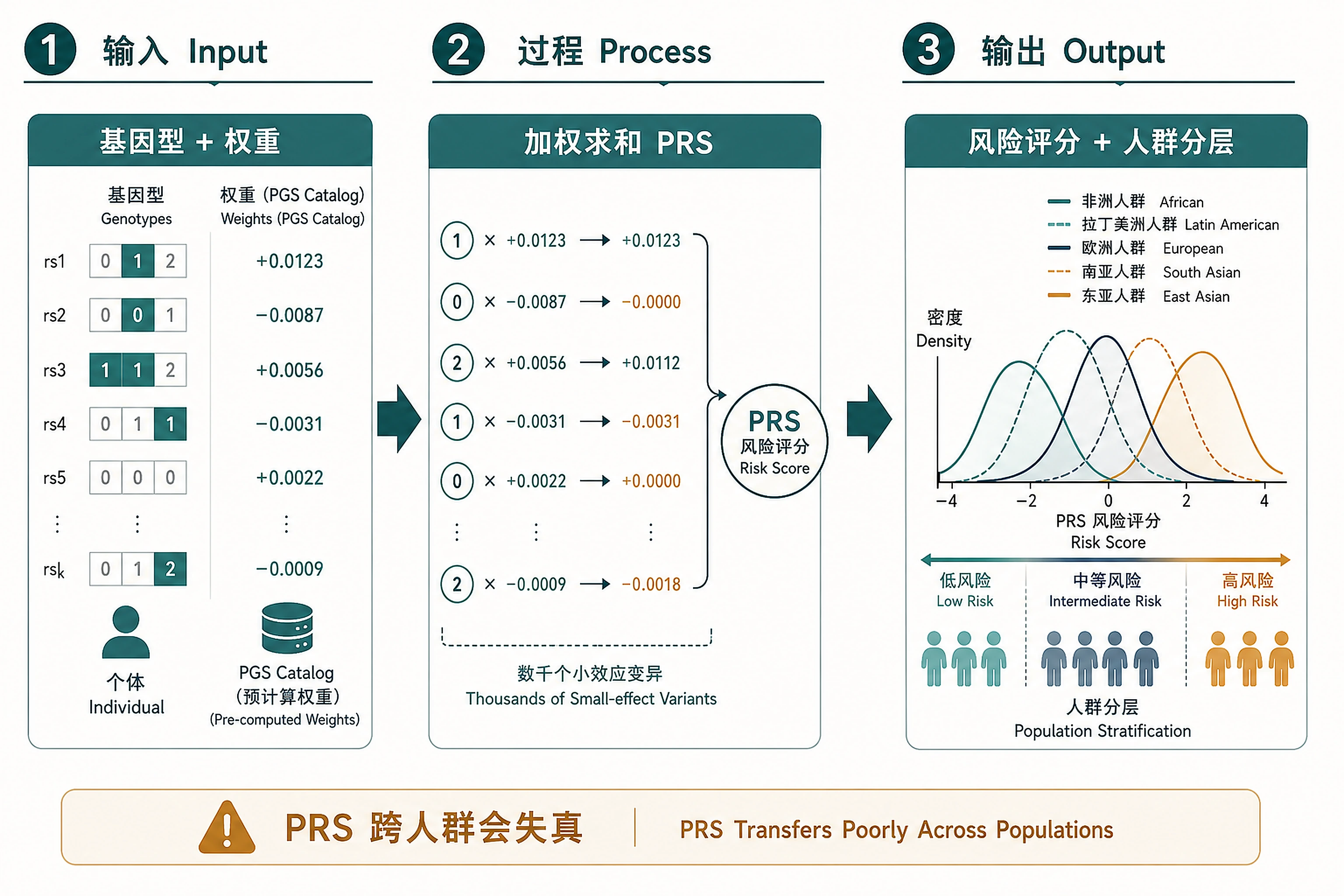
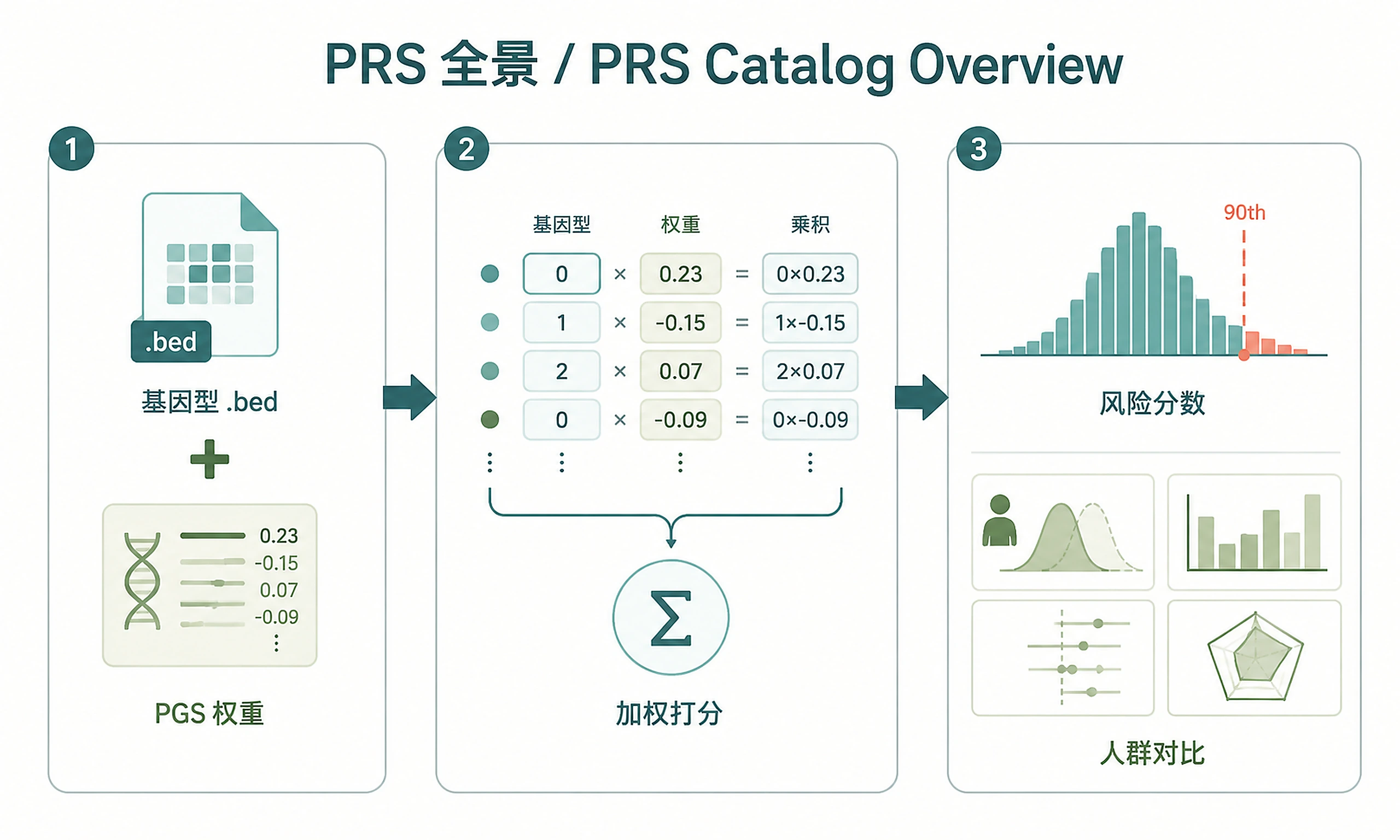
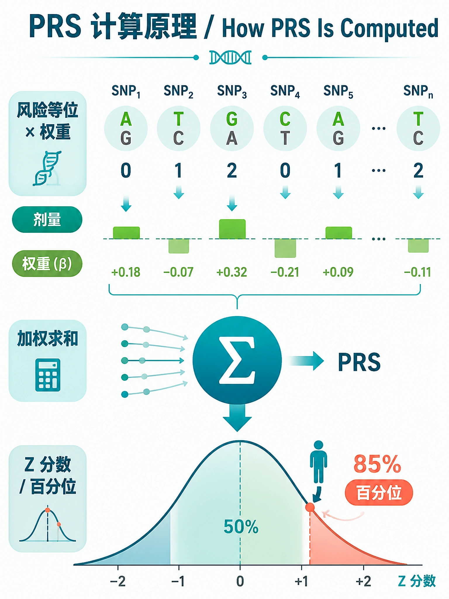
Problem. Sum thousands of small-effect variants into one risk score.
Learning goals
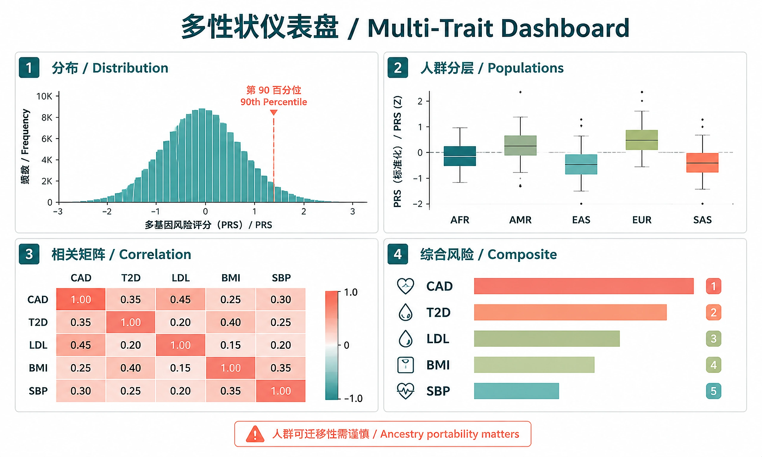
- Complex traits are the sum of many small effects
- PRS is strongly ancestry-specific
Figures
Tutorial
When to Use This Skill
- You have a trait of interest and want to calculate PRS using published, peer-reviewed weights
- Multi-trait risk profiling (e.g., cardiometabolic panel: CAD, T2D, LDL, BMI, blood pressure)
- Population comparisons of genetic risk across ancestry groups
- No GWAS summary statistics needed — uses pre-computed weights from PGS Catalog
- Quick PRS — minutes per trait (download + score), no LD computation required
For de novo PRS from raw GWAS summary statistics, use the polygenic-risk-score skill (LDpred2-auto) instead.
Installation
install.packages(c("data.table", "ggplot2", "ggprism", "dplyr", "R.utils", "jsonlite", "remotes"))
remotes::install_github("privefl/bigsnpr")
| Software | Version | License | Commercial Use | Install |
|---|---|---|---|---|
| bigsnpr | ≥1.12 | GPL-3 | ✅ Permitted | remotes::install_github("privefl/bigsnpr") |
| data.table | ≥1.14 | MPL-2.0 | ✅ Permitted | install.packages('data.table') |
| ggplot2 | ≥3.4 | MIT | ✅ Permitted | install.packages('ggplot2') |
| ggprism | ≥1.0.3 | GPL (≥3) | ✅ Permitted | install.packages('ggprism') |
| dplyr | ≥1.1 | MIT | ✅ Permitted | install.packages('dplyr') |
| jsonlite | ≥1.8 | MIT | ✅ Permitted | install.packages('jsonlite') |
| R.utils | ≥2.12 | LGPL (≥2.1) | ✅ Permitted | install.packages('R.utils') |
Inputs
- Target genotypes: PLINK binary format (.bed/.bim/.fam) — or use 1000 Genomes Phase 3 example data (2,490 individuals, 5 super-populations)
- PGS Catalog score IDs: One or more PGS IDs (e.g.,
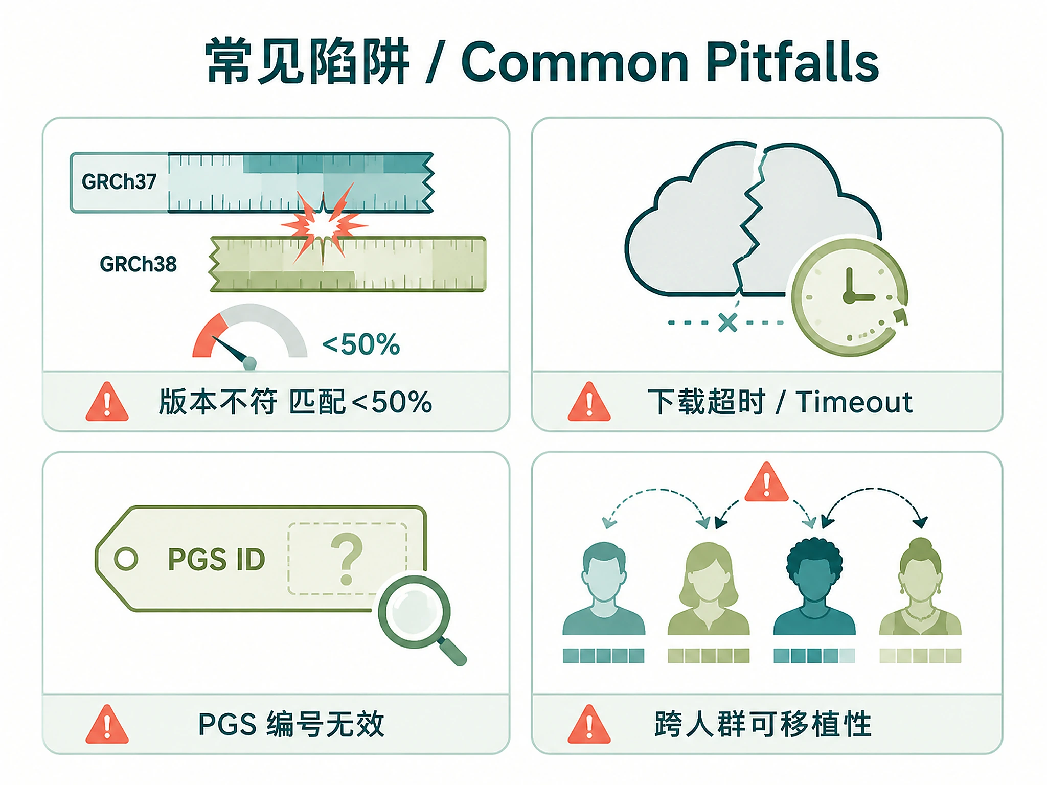
PGS000018for CAD) — usesearch_pgs_catalog()to discover available scores - Genome build: GRCh37 (default, matches 1000 Genomes) or GRCh38
Outputs
Per-trait files:
prs_scores_<trait>.csv— Individual PRS (z-scores, percentiles, population labels)distribution_<trait>.png/svg— PRS distribution histogrampopulation_<trait>.png/svg— PRS by super-population boxplot
Combined files:
combined_prs_scores.csv— All individuals x all traits (wide format) + composite riskprs_correlation_matrix.csv— Trait-trait PRS correlation matrixpopulation_summary.csv— Mean PRS by super-population per traitmatch_reports.csv— Variant matching summary per trait
Dashboard plots:
dashboard_correlation_matrix.png/svg— Heatmap of trait PRS correlationsdashboard_composite_risk.png/svg— Composite risk distribution by populationdashboard_population_heatmap.png/svg— Mean PRS by trait x super-population
Analysis objects (RDS):
prs_analysis.rds— Complete analysis object for downstream use- Load with:
obj <- readRDS('prs_analysis.rds') - Contains: combined_scores, per_trait, cor_matrix, match_reports, snp_weights, trait_info
Clarification Questions
-
Input Data (ASK THIS FIRST):
- Do you have specific genotype files (.bed/.bim/.fam) to score?
- Or use 1000 Genomes Phase 3 example data? (2,490 individuals, 26 populations, 5 super-populations)
-
Traits to Score:
- (If using example data) The demo scores 5 cardiometabolic traits (CAD, T2D, LDL, BMI, SBP). Choose analysis mode:
- a) Full cardiometabolic panel — all 5 traits (recommended)
- b) Select specific traits from the panel
- (If using your own data) What traits do you want to score? Use
search_pgs_catalog("trait name")to find PGS IDs.
-
Analysis Options:
- a) Standard analysis with dashboard (recommended)
- b) Individual trait scoring only (no dashboard)
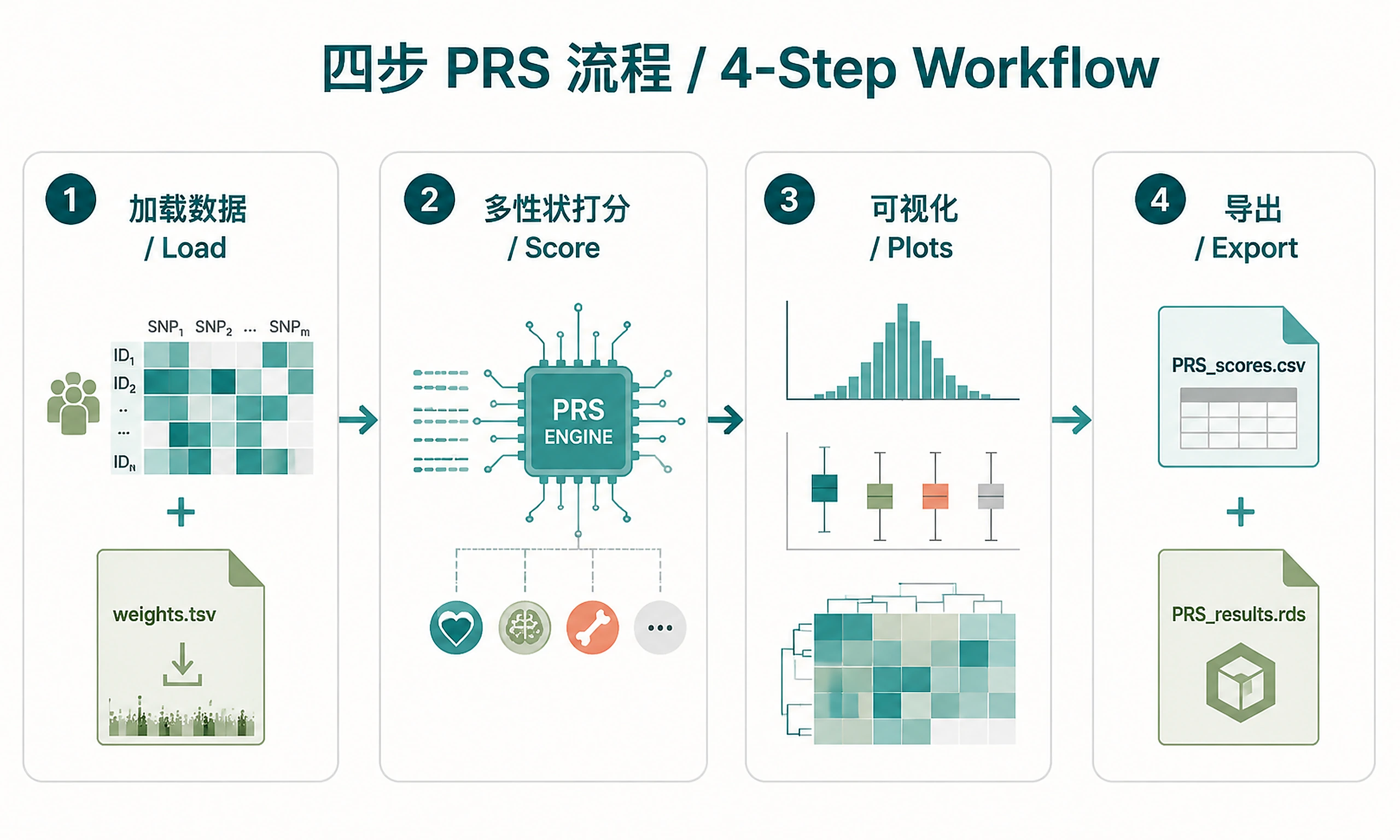
Standard Workflow
🚨 MANDATORY: USE SCRIPTS EXACTLY AS SHOWN - DO NOT WRITE INLINE CODE 🚨
Step 1 - Load reference genotypes and PGS weights:
source("scripts/load_reference_data.R")
ref_data <- load_reference_data()

source("scripts/load_pgs_weights.R")
trait_weights <- load_demo_weights()
DO NOT write custom download or parsing code. Use the scripts.
Step 2 - Score all traits:
source("scripts/score_traits.R")
DO NOT write inline scoring code (big_prodVec, allele matching, etc.). Just source the script.
Step 3 - Generate visualizations:
source("scripts/generate_plots.R")
generate_all_plots(all_results, output_dir = "results")
DO NOT write inline plotting code (ggsave, ggplot, geom_tile, etc.). Just use the script.
The script handles PNG + SVG export with graceful fallback for SVG dependencies.
Step 4 - Export results:
source("scripts/export_results.R")
export_all(all_results, output_dir = "results")
DO NOT write custom export code. Use export_all().
✅ VERIFICATION - You should see:
- After Step 1:
"✓ Reference data loaded successfully"and"✓ PGS Catalog weights loaded: 5/5 traits" - After Step 2:
"✓ Multi-trait PRS scoring completed successfully! (5 traits, 2490 individuals)" - After Step 3:
"✓ All plots generated successfully!" - After Step 4:
"=== Export Complete ==="
❌ IF YOU DON'T SEE THESE: You wrote inline code. Stop and use source().
⚠️ CRITICAL - DO NOT:
- ❌ Write inline scoring code → STOP: Use
source("scripts/score_traits.R") - ❌ Write inline plotting code (ggsave, ggplot, etc.) → STOP: Use
generate_all_plots() - ❌ Write custom export code → STOP: Use
export_all() - ❌ Try to install svglite → script handles SVG fallback automatically
⚠️ IF SCRIPTS FAIL - Script Failure Hierarchy:
- Fix and Retry (90%) — Install missing package, re-run script
- Modify Script (5%) — Edit the script file itself, document changes
- Use as Reference (4%) — Read script, adapt approach, cite source
- Write from Scratch (1%) — Only if genuinely impossible, explain why
NEVER skip directly to writing inline code without trying the script first.
Scoring Custom Traits
To score a single custom trait instead of the demo panel:
source("scripts/load_reference_data.R")
ref_data <- load_reference_data()

source("scripts/load_pgs_weights.R")
# Search for available scores
scores <- search_pgs_catalog("your trait name")
# Download specific score
trait_weights <- list()
tw <- download_pgs_weights("PGS_ID_HERE")
trait_weights[["TRAIT"]] <- list(
    weights = tw$weights, pgs_id = tw$pgs_id, score_meta = tw$score_meta,
    trait_name = "Your Trait", short_name = "TRAIT"
)

# Then continue with Steps 2-4 as above
source("scripts/score_traits.R")
Common Issues
| Error | Cause | Solution |
|---|---|---|
| "bigsnpr not found" | Missing core dependency | remotes::install_github("privefl/bigsnpr") |
| Download timeout | Large scoring file or slow connection | Set options(timeout = 900) before running Step 1 |
| Low match rate (<50%) | Genome build mismatch | Ensure PGS weights and genotypes use same build (GRCh37 for 1000G) |
| PGS ID not found | Wrong or deprecated PGS ID | Use search_pgs_catalog("trait") to find valid IDs |
| SVG export error | Missing optional dependency | generate_all_plots() handles fallback automatically. DO NOT install svglite manually. |
| "catalog_data not found" | Wrong script for this skill | Use score_traits.R (not pgs_catalog_scoring.R from the LDpred2 skill) |
| Memory error during scoring | Very large scoring file | Normal for genome-wide scores. Ensure ≥8GB RAM available. |
Suggested Next Steps
After completing multi-trait PRS:
- Downstream analysis — Load
prs_analysis.rdsfor custom analyses - Additional traits — Add more PGS scores to expand the risk panel
- De novo PRS — Use
polygenic-risk-scoreskill for traits without PGS Catalog scores - GWAS interpretation — Pair with functional annotation skills
Related Skills
polygenic-risk-score— De novo PRS using LDpred2-auto (requires GWAS summary statistics)eqtl-colocalization-coloc— Colocalization of GWAS signals with eQTLs
References
- Lambert SA, et al. (2021). The Polygenic Score Catalog as an open database for reproducibility and systematic evaluation. Nature Genetics, 53(4), 420-425.
- 1000 Genomes Project Consortium (2015). A global reference for human genetic variation. Nature, 526(7571), 68-74.
- Privé F, et al. (2022). Portability of 245 polygenic scores when derived from the UK Biobank and applied to 9 ancestry groups from the same cohort. AJHG, 109(1), 12-23.
- Khera AV, et al. (2018). Genome-wide polygenic scores for common diseases identify individuals with risk equivalent to monogenic mutations. Nature Genetics, 50(9), 1219-1224.
- PGS Catalog: https://www.pgscatalog.org/
Code preview
scripts/export_results.R
###############################################################################
# export_results.R — Export multi-trait PRS results and RDS for downstream use
#
# Function:
#   export_all(all_results, output_dir)
###############################################################################

library(data.table)
library(dplyr)

# --- Helper: population summary -----------------------------------------------

.make_population_summary <- function(combined_scores) {
    if (!"super_population" %in% names(combined_scores)) return(NULL)

    prs_cols <- grep("^prs_", names(combined_scores), value = TRUE)
    trait_labels <- sub("^prs_", "", prs_cols)

    rows <- list()
    for (i in seq_along(prs_cols)) {
        s <- combined_scores %>%
            filter(!is.na(super_population)) %>%
            group_by(super_population) %>%
            summarise(
                n = n(),
                mean_z = round(mean(.data[[prs_cols[i]]], na.rm = TRUE), 4),
                sd_z = round(sd(.data[[prs_cols[i]]], na.rm = TRUE), 4),
                min_z = round(min(.data[[prs_cols[i]]], na.rm = TRUE), 4),
                max_z = round(max(.data[[prs_cols[i]]], na.rm = TRUE), 4),
                .groups = "drop"
            ) %>%
            mutate(trait = trait_labels[i])
        rows[[i]] <- s
    }

    # Add composite risk summary
    comp_s <- combined_scores %>%
        filter(!is.na(super_population)) %>%
        group_by(super_population) %>%
        summarise(
            n = n(),
            mean_z = round(mean(composite_risk, na.rm = TRUE), 4),
            sd_z = round(sd(composite_risk, na.rm = TRUE), 4),
            min_z = round(min(composite_risk, na.rm = TRUE), 4),
            max_z = round(max(composite_risk, na.rm = TRUE), 4),
            .groups = "drop"
        ) %>%
        mutate(trait = "COMPOSITE")
    rows[[length(rows) + 1]] <- comp_s

    do.call(rbind, rows)
}

# --- Main export function -----------------------------------------------------

#' Export all multi-trait PRS results
#' @param all_results list from score_traits.R
#' @param output_dir Directory to save files (default: "results")
export_all <- function(all_results, output_dir = "results") {
    cat("\n=== Exporting Multi-Trait PRS Results ===\n\n")

    dir.create(output_dir, showWarnings = FALSE, recursive = TRUE)

    # 1. Combined scores (wide format: one row per individual, one column per trait)
    cat("[1/7] Combined PRS scores (wide format)\n")
    fwrite(all_results$combined_scores, file.path(output_dir, "combined_prs_scores.csv"))
    cat("  Saved:", file.path(output_dir, "combined_prs_scores.csv"), "\n")
    cat("  (", nrow(all_results$combined_scores), " individuals x ",
        all_results$n_traits, " traits)\n\n", sep = "")

    # 2. Per-trait scores (individual CSVs)
    cat("[2/7] Per-trait PRS scores\n")
    for (trait_name in all_results$trait_names) {
        fname <- paste0("prs_scores_", tolower(trait_name), ".csv")
        fwrite(all_results$per_trait[[trait_name]], file.path(output_dir, fname))
        cat("  Saved:", file.path(output_dir, fname), "\n")
    }
    cat("\n")

    # 3. Correlation matrix
scripts/generate_plots.R
###############################################################################
# generate_plots.R — Multi-trait PRS visualizations using ggprism
#
# Per-trait plots:
#   plot_trait_distribution()      — Histogram for one trait
#   plot_trait_population()        — Boxplot by super-population for one trait
#
# Dashboard plots:
#   plot_correlation_heatmap()     — Trait-trait PRS correlation matrix
#   plot_composite_risk()          — Composite risk distribution by population
#   plot_population_heatmap()      — Mean PRS by trait x super-population
#
# Orchestrator:
#   generate_all_plots(all_results, output_dir)
###############################################################################

library(ggplot2)
library(ggprism)
library(dplyr)

# --- SVG support (optional, graceful fallback) --------------------------------

.has_svglite <- requireNamespace("svglite", quietly = TRUE)
if (.has_svglite) library(svglite)

# --- Save helper (PNG + SVG always) -------------------------------------------

.save_plot <- function(plot, base_path, width = 8, height = 6, dpi = 300) {
    png_path <- sub("\\.(svg|png)$", ".png", base_path)
    ggsave(png_path, plot = plot, width = width, height = height, dpi = dpi, device = "png")
    cat("   Saved:", png_path, "\n")

    svg_path <- sub("\\.(svg|png)$", ".svg", base_path)
    tryCatch({
        ggsave(svg_path, plot = plot, width = width, height = height, device = "svg")
        cat("   Saved:", svg_path, "\n")
    }, error = function(e) {
        tryCatch({
            svg(svg_path, width = width, height = height)
            print(plot)
            dev.off()
            cat("   Saved:", svg_path, "\n")
        }, error = function(e2) {
            cat("   (SVG export failed - PNG available)\n")
        })
    })
}

# Super-population color palette (consistent across all plots)
.pop_colors <- c(
    "AFR" = "#E74C3C", "AMR" = "#F39C12", "EAS" = "#2ECC71",
    "EUR" = "#3498DB", "SAS" = "#9B59B6"
)

# --- Per-trait: PRS Distribution ----------------------------------------------

plot_trait_distribution <- function(scores, trait_name, output_dir = "results") {
    p <- ggplot(scores, aes(x = prs_zscore)) +
        geom_histogram(aes(y = after_stat(density)),
                       bins = 30, fill = "#4A90D9", color = "white", alpha = 0.8) +
        geom_density(color = "#2C3E50", linewidth = 0.8) +
        geom_vline(xintercept = 0, linetype = "dashed", color = "#E67E22", linewidth = 0.8) +
        labs(
            title = paste(trait_name, "- PRS Distribution"),
            subtitle = paste(nrow(scores), "individuals from 1000 Genomes Phase 3"),
            x = "PRS (Z-score)",
            y = "Density"
        ) +
        theme_prism(base_size = 12) +
        theme(plot.title = element_text(hjust = 0.5, face = "bold", size = 14),
              plot.subtitle = element_text(hjust = 0.5, size = 10, color = "gray40"))

    fname <- paste0("distribution_", gsub(" ", "_", tolower(trait_name)), ".png")
    .save_plot(p, file.path(output_dir, fname), width = 8, height = 6)
    return(invisible(p))
}

# --- Per-trait: Population Comparison -----------------------------------------

plot_trait_population <- function(scores, trait_name, output_dir = "results") {
scripts/load_pgs_weights.R
###############################################################################
# load_pgs_weights.R — Search PGS Catalog and download scoring weights
#
# Functions:
#   search_pgs_catalog(trait)      — Search for available PGS scores by trait
#   download_pgs_weights(pgs_id)   — Download a single harmonized scoring file
#   get_demo_traits()              — Get cardiometabolic demo trait configuration
#   load_demo_weights(data_dir)    — Download all 5 cardiometabolic demo weights
###############################################################################

library(data.table)

if (!requireNamespace("jsonlite", quietly = TRUE)) {
    install.packages("jsonlite")
}

`%||%` <- function(a, b) if (!is.null(a)) a else b

# --- Search PGS Catalog ------------------------------------------------------

#' Search PGS Catalog for available scores by trait name
#' @param trait Character string (e.g. "coronary artery disease", "BMI", "LDL cholesterol")
#' @return data.frame of matching scores with id, name, trait, variants, method, publication
search_pgs_catalog <- function(trait) {
    cat("Searching PGS Catalog for '", trait, "'...\n", sep = "")

    trait_url <- paste0("https://www.pgscatalog.org/rest/trait/search?term=",
                        utils::URLencode(trait))
    trait_resp <- jsonlite::fromJSON(trait_url, flatten = TRUE)

    if (length(trait_resp$results) == 0) {
        cat("  No traits found matching '", trait, "'\n", sep = "")
        return(data.frame())
    }

    all_pgs_ids <- unique(unlist(trait_resp$results$associated_pgs_ids))
    if (length(all_pgs_ids) == 0) {
        cat("  Traits found but no associated PGS scores\n")
        return(data.frame())
    }

    cat("  Found", length(all_pgs_ids), "scores across",
        nrow(trait_resp$results), "matching traits\n\n")

    # Fetch details for top scores (limit to first 20 to avoid rate limiting)
    fetch_ids <- head(all_pgs_ids, 20)
    scores <- do.call(rbind, lapply(fetch_ids, function(pgs_id) {
        score_url <- paste0("https://www.pgscatalog.org/rest/score/", pgs_id)
        tryCatch({
            s <- jsonlite::fromJSON(score_url, flatten = TRUE)
            data.frame(
                pgs_id = s$id,
                name = s$name %||% NA_character_,
                trait = s$trait_reported %||% NA_character_,
                variants = s$variants_number %||% NA_integer_,
                method = s$method_name %||% NA_character_,
                genome_build = s$variants_genomebuild %||% NA_character_,
                publication = paste0(s$publication$firstauthor %||% "Unknown",
                                     " (", substr(s$publication$date_publication %||% "", 1, 4), ")"),
                stringsAsFactors = FALSE
            )
        }, error = function(e) NULL)
    }))

    if (is.null(scores) || nrow(scores) == 0) {
        cat("  Could not fetch score details\n")
        return(data.frame())
    }

    cat("  Available PGS scores:\n")
    cat("  ", paste(rep("-", 80), collapse = ""), "\n")
    for (i in seq_len(min(nrow(scores), 15))) {
        cat(sprintf("  %s | %s variants | %s | %s\n",
                    scores$pgs_id[i],
                    format(scores$variants[i], big.mark = ","),
                    scores$method[i] %||% "N/A",
                    scores$publication[i]))
    }
    if (nrow(scores) > 15) cat("  ... and", nrow(scores) - 15, "more\n")
    cat("  ", paste(rep("-", 80), collapse = ""), "\n\n")
Companion files
| Type | Path | Bytes |
|---|---|---|
| Markdown | references/interpretation-guide.md | 2,911 |
| Markdown | references/pgs-catalog-guide.md | 3,481 |
| R | scripts/export_results.R | 8,008 |
| R | scripts/generate_plots.R | 12,115 |
| R | scripts/load_pgs_weights.R | 9,155 |
| R | scripts/load_reference_data.R | 7,122 |
| R | scripts/score_traits.R | 7,703 |
| Markdown | SKILL.md | 8,809 |
| JSON | skill.meta.json | 1,892 |