DESeq2 Differential Expression
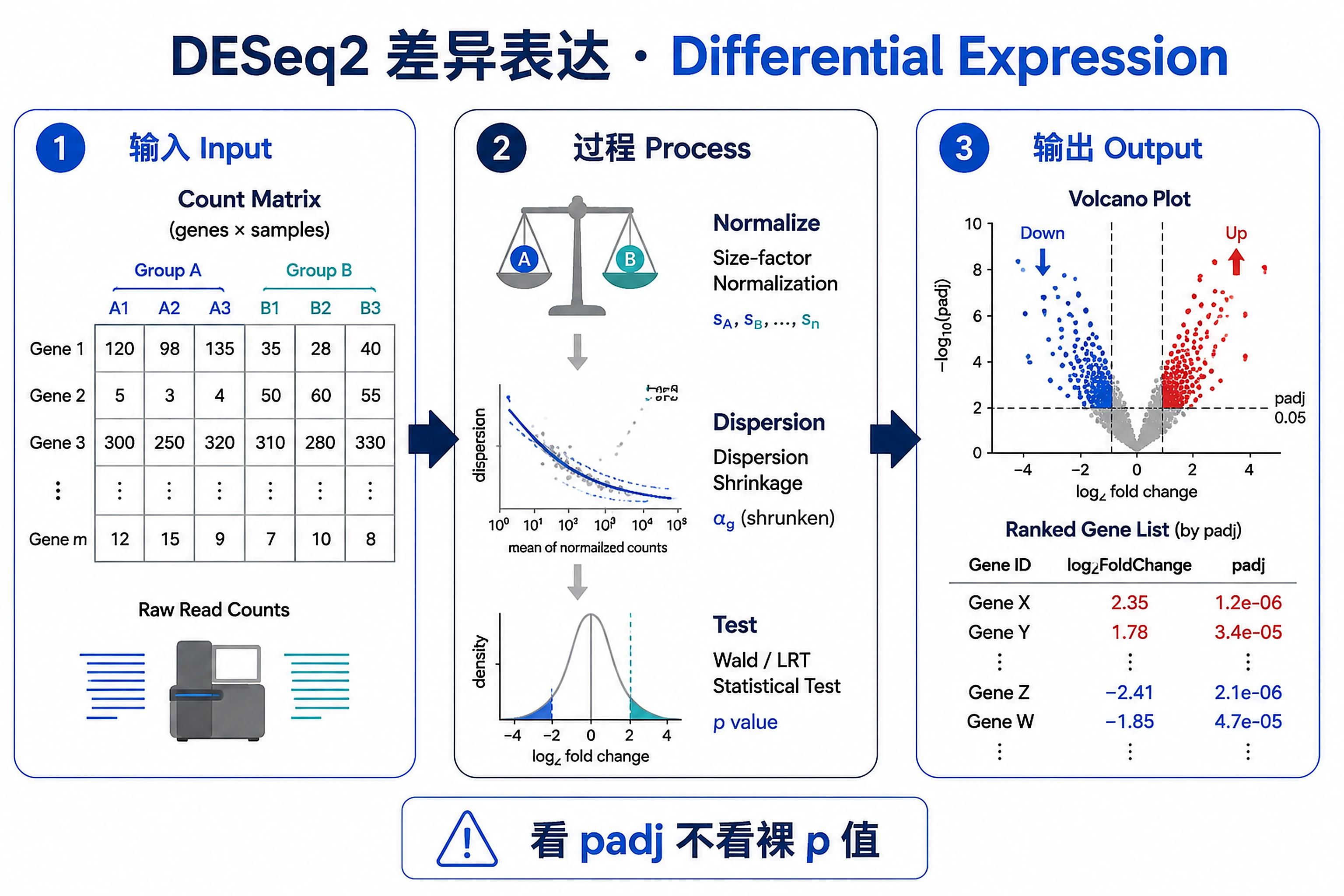
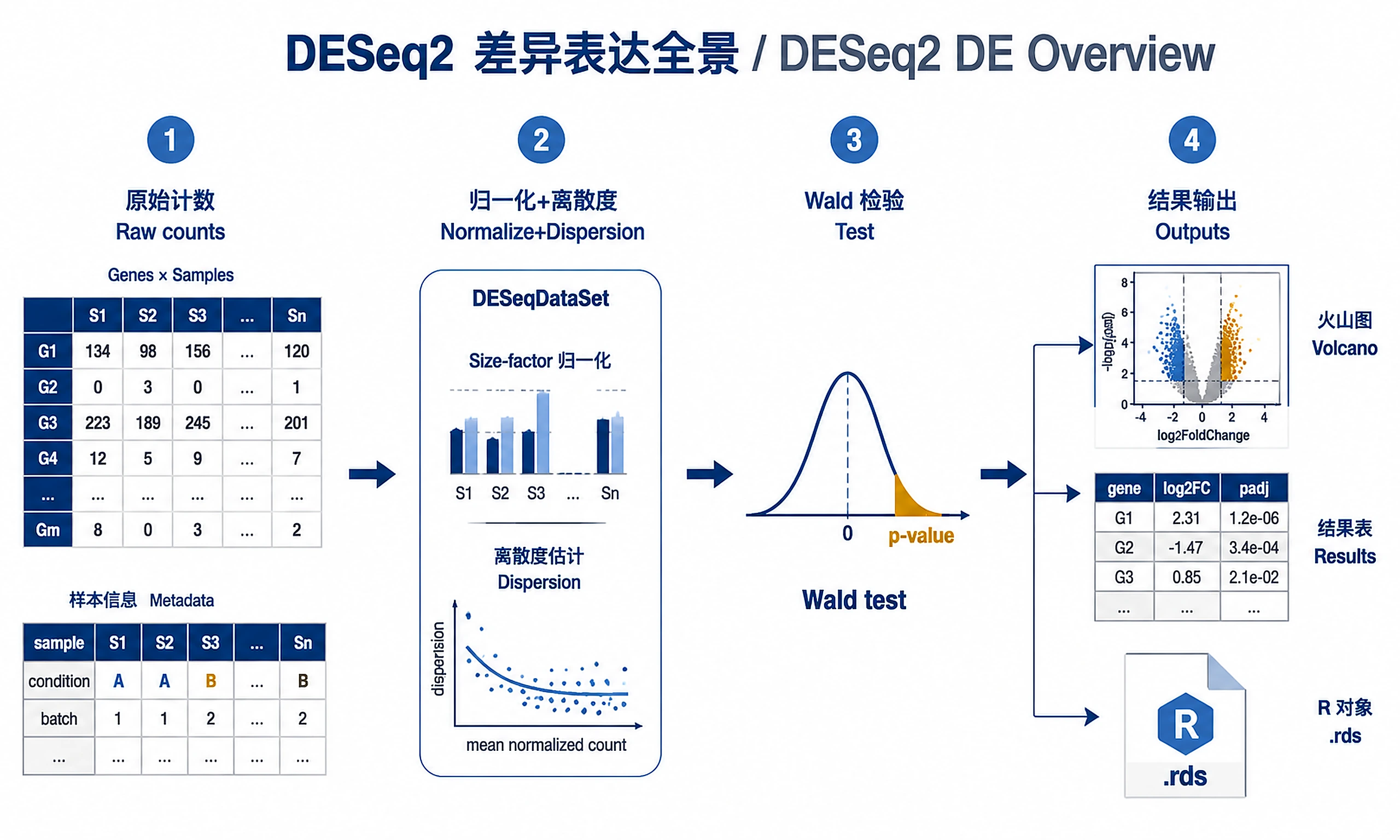
Differential expression from raw counts with DESeq2 — the classic entry workflow.
Overview
Problem. Given an integer gene×sample count matrix, find genes significantly up/down between groups.
Learning goals
- Why DE needs raw counts, not TPM (negative-binomial model)
- Judge significance by padj, not the raw p-value
Figures
Tutorial
Core DESeq2 workflow for RNA-seq differential expression analysis with count data.
When to Use This Skill
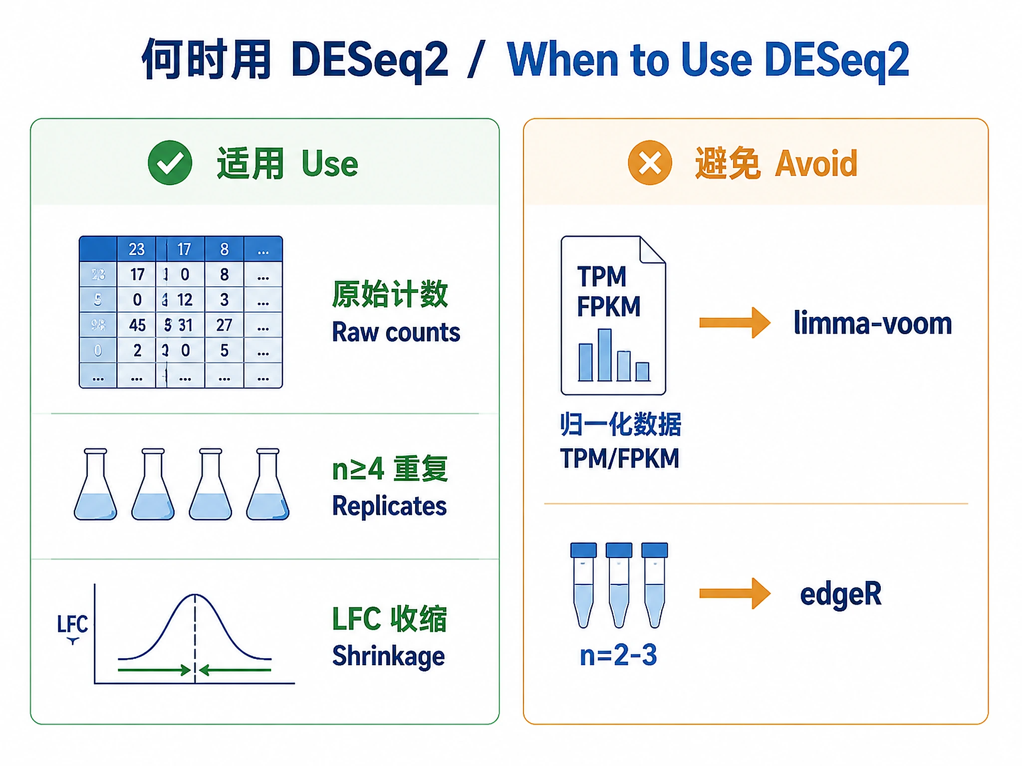
Use DESeq2 when you have:
- ✅ Raw integer count data (not normalized TPM/FPKM)
- ✅ Biological replicates (≥2 per condition, ≥4 recommended)
- ✅ Need for log fold change shrinkage (ranking/visualization)
- ✅ Medium to large sample sizes (DESeq2's strength)
Don't use DESeq2 for:
- ❌ Normalized data (TPM/FPKM) → use limma-voom instead
- ❌ Very small samples (n=2-3) → consider edgeR quasi-likelihood
Quick Start (Example Data)
Test this skill with real RNA-seq data in ~2 minutes:
source("scripts/load_example_data.R")
data <- load_pasilla_data()  # Auto-installs pasilla package if needed (~2 min, ~50MB)
counts <- data$counts        # 14,599 genes × 7 samples
coldata <- data$coldata      # Metadata: treated vs untreated

# Run complete workflow
source("scripts/basic_workflow.R")  # Creates dds, res, resLFC objects + prints summary
What you get:
- Dataset: Drosophila pasilla gene RNAi knockdown (Brooks et al. 2011)
- Comparison: 3 treated vs 4 untreated samples
- Expected results: ~1,000 significant genes at padj < 0.1
For your own data: Replace data loading with your count matrix and metadata (see Inputs section).
Installation
Core packages (required):
# Set CRAN mirror first (required for installation)
options(repos = c(CRAN = "https://cloud.r-project.org"))

if (!require('BiocManager', quietly = TRUE))
    install.packages('BiocManager')
BiocManager::install(c('DESeq2', 'apeglm'))
Example data packages (optional - for testing/learning):
BiocManager::install(c('pasilla', 'airway')) # ~70MB total, ~2-3 min
Visualization packages (required for QC plots):
# For publication-quality plots (required - generates PNG)
install.packages(c('ggplot2', 'ggprism', 'ggrepel'))

# For SVG export (optional - generates both PNG + SVG)
install.packages('svglite')
License: LGPL (>= 3) (commercial use permitted)
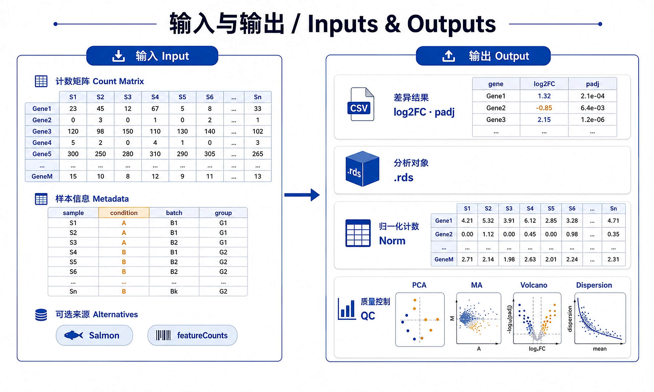
Inputs
Required:
- Count matrix: Raw integer counts (genes × samples)
- Rows = genes (any identifier: Ensembl, symbols, etc.)
- Columns = samples
- Values = non-negative integers
- Sample metadata: Data frame with sample information
- Row names must match count matrix column names
- Required column:
condition(factor with 2+ levels) - Optional: batch, covariates for complex designs
Alternative inputs:
- Salmon/Kallisto output (via tximport)
- SummarizedExperiment object
- featureCounts/HTSeq output
- Bioconductor data packages (pasilla, airway)
See references/deseq2-reference.md for loading examples.
Outputs
Primary results:
deseq2_results.csv- Full differential expression table (baseMean, log2FC, lfcSE, pvalue, padj)deseq2_results_shrunk.csv- Shrunken LFC for visualization/rankingdds_object.rds- DESeqDataSet for further analysis
Normalized data:
normalized_counts.csv- Size-factor normalized countsvst_transformed.csv/rlog_transformed.csv- Variance-stabilized values
QC plots (PNG always, SVG strongly preferred, 300 DPI):
dispersion_plot.png/.svg- Dispersion estimates vs meanpca_plot.png/.svg- Principal component analysisma_plot.png/.svg- Mean-average plotvolcano_plot.png/.svg- Volcano plot (log2FC vs -log10 padj)- ⚠️ SVG requires
svglitepackage:install.packages('svglite')(falls back to PNG-only if unavailable)
Clarification Questions
⚠️ CRITICAL: Always ask question #1 first to check if user has provided input files before proceeding with analysis.
Before starting, gather:
-
Input Files (ASK THIS FIRST):
- Do you have specific count matrix file(s) to analyze?
- If uploaded: Is this the count matrix (genes × samples, raw integer counts)?
- Expected formats: CSV/TSV, RDS (SummarizedExperiment), Salmon/Kallisto output
- Or use example data for testing?
- Use
source("scripts/load_example_data.R"); data <- load_pasilla_data() - Requires installing
pasillapackage (~2 min, ~50MB) - ⚠️ If data is normalized (TPM/FPKM): Use limma-voom skill instead
-
Sample Metadata (if using own data):
- What is the primary comparison (e.g., treated vs control)?
- Which group is the reference/control?
- Any covariates to adjust for (batch, sex, sequencing run)?
- Validation: Confirm sample IDs match between count matrix columns and metadata rows
-
Experimental Design:
- Simple:
~ condition| Multi-factor:~ batch + condition| Paired:~ individual + condition| Interaction:~ genotype * treatment - See references/decision-guide.md#design-formulas
- Simple:
-
Sample Size Check:
- n ≥ 4 per group (recommended) | n = 2-3 (consider edgeR) | n < 2 (insufficient)
-
Significance Thresholds:
- Standard: padj < 0.05, |log2FC| ≥ 1 | Relaxed: padj < 0.1 | Stringent: padj < 0.01, |log2FC| ≥ 2
-
Analysis Goals:
- Single pairwise comparison or multiple comparisons?
- Need visualizations (volcano, heatmap)? → Use de-results-to-plots skill after
- Need gene annotations? → Use de-results-to-gene-lists skill after
Typical Complete Workflow
This skill performs core differential expression analysis with QC plots. For a complete RNA-seq workflow:
- This skill: Run DESeq2 → get
dds,res, normalized counts, QC plots (PCA, MA, volcano, dispersion) - de-results-to-gene-lists: Filter significant genes → add annotations → export
- de-results-to-plots (optional): Advanced visualizations (heatmaps, custom plots)
Quick start: "Run DESeq2 analysis and filter significant genes with annotations"
Why separate skills? Modular design works across DE methods (DESeq2, edgeR, limma). See Suggested Next Steps for details.
Standard Workflow
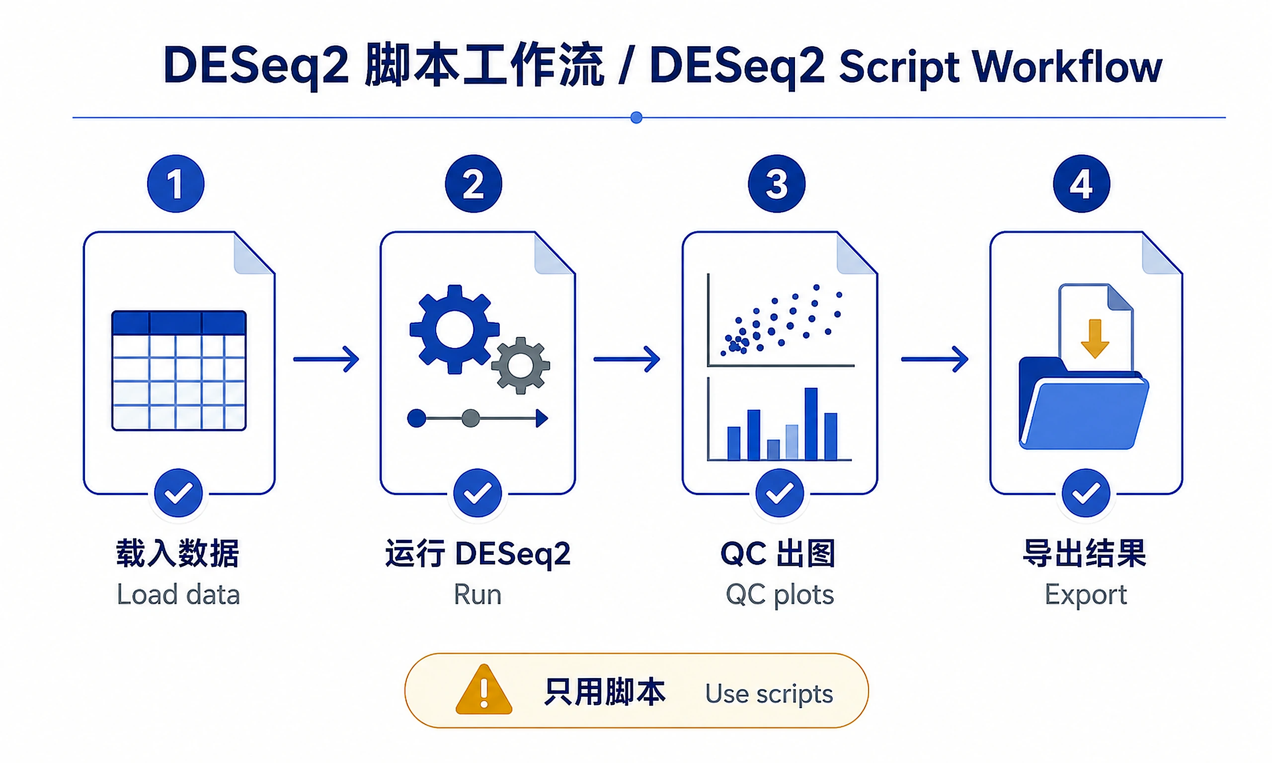
🚨 MANDATORY: USE SCRIPTS EXACTLY AS SHOWN - DO NOT WRITE INLINE CODE 🚨
This skill uses low-freedom script execution. You must:
- ✅ Source the scripts using the exact commands below
- ✅ Wait for confirmation messages after each step
- ❌ NOT write inline DESeq2 code
- ❌ NOT rewrite plotting code
- ❌ NOT modify commands unless explicitly adapting for user-specific data
WHY USE SCRIPTS: They handle package installation, data validation, sample ID fixes, and error checking automatically. Writing inline code wastes time, introduces errors, and violates the skill design.
Step 1 - Load example data:
source("scripts/load_example_data.R")
data <- load_pasilla_data()
counts <- data$counts
coldata <- data$coldata
Step 2 - Run DESeq2 analysis:
source("scripts/basic_workflow.R")
DO NOT expand this into inline code. DO NOT write the DESeq2 steps manually. Just source the script.
Step 3 - Generate QC plots:
source("scripts/qc_plots.R")
run_all_qc(dds, res, output_dir = "results")
DO NOT write inline plotting code (ggsave, plotMA, etc.). Just source the script.
The script handles PNG + SVG export with graceful fallback for SVG dependencies.
Step 4 - Export results:
source("scripts/export_results.R")
export_all(dds, res, resLFC, output_dir = "results")
DO NOT write custom export code. Use export_all() to save all standard outputs including RDS and transformed counts.
✅ VERIFICATION - You should see these messages:
- After Step 1:
"✓ Pasilla dataset loaded successfully"with dimensions - After Step 2:
"✓ Basic workflow completed successfully!"with summary statistics - After Step 3:
"✓ All QC plots generated successfully!"with file names - After Step 4:
"=== Export Complete ==="with list of 6-7 files saved
❌ IF YOU DON'T SEE THESE MESSAGES: You wrote inline code instead of using source(). Stop and use the commands above.
⚠️ CRITICAL - DO NOT:
- ❌ Write inline data loading code → STOP: This violates the skill design. Use
source("scripts/load_example_data.R")instead. Inline loading causes sample ID mismatches and missing validations. - ❌ Write inline DESeq2 workflow code → STOP: This violates the skill design. Use
source("scripts/basic_workflow.R")instead. Inline workflow wastes time and introduces bugs. - ❌ Write inline plotting code (ggsave, plotMA, etc.) → STOP: This violates the skill design. Use
source("scripts/qc_plots.R")andrun_all_qc()instead. If scripts fail, fix the script, don't rewrite inline. - ❌ Write custom export code → STOP: This violates the skill design. Use
source("scripts/export_results.R")andexport_all()instead. Custom export code misses RDS objects and transformed counts needed downstream. - ❌ Try to install svglite → script handles SVG fallback automatically
- ❌ Use absolute paths for scripts → Always use relative paths
scripts/file.R - ❌ WRONG:
source("/mnt/knowhow/workflows/bulk-rnaseq-counts-to-de-deseq2/scripts/load_example_data.R") - ❌ WRONG:
setwd("/absolute/path/to/skill") - ✅ CORRECT:
source("scripts/load_example_data.R")(skill should already be working directory)
⚠️ IF SCRIPTS FAIL - Script Failure Hierarchy:
- Fix and Retry (90%) - Install missing package, re-run script
- Modify Script (5%) - Edit the script file itself, document changes
- Use as Reference (4%) - Read script, adapt approach, cite source
- Write from Scratch (1%) - Only if genuinely impossible, explain why
NEVER skip directly to writing inline code without trying the script first.
📁 Output Directory Paths:
- ✅ Recommended: Use relative paths like
output_dir = "results"(creates folder in working directory) - ✅ Also valid: Environment-specific absolute paths like
output_dir = "/mnt/results"(containerized environments only)
✅ When to read references for adaptation (NOT rewriting):
- Design formulas (multi-factor, interactions): Read references/comprehensive-reference.md#design-formulas to understand patterns
- Result extraction (specific contrasts): Read references/comprehensive-reference.md#extracting-results
- Shrinkage methods (ashr vs apeglm): Read references/comprehensive-reference.md#log-fold-change-shrinkage
❌ When NOT to write custom inline code:
- Unless user explicitly says: "show me the complete inline workflow without using scripts"
- The scripts already handle 95% of use cases - use them first, customize only if truly needed
What the scripts provide:
- scripts/load_example_data.R -
load_pasilla_data(),load_airway_data(),validate_input_data() - scripts/basic_workflow.R - Complete DESeq2 pipeline with validation and error messages
- scripts/qc_plots.R - Publication-quality plots with ggplot2/ggprism/ggrepel (PNG + SVG if svglite installed)
- scripts/export_results.R -
export_all()saves all outputs (CSV, RDS, transformed counts)
When Scripts Fail
When a script fails, follow this hierarchy:
1. Fix and Retry (Preferred)
- Read the error message - Understand what went wrong
- Install missing packages - Use
BiocManager::install()orinstall.packages() - Update dependencies - If version conflicts, update packages:
install.packages('package_name') - Check your data - Ensure count matrices are integer counts and metadata is properly formatted
- Re-run the script - After fixing the issue, source the script again
2. Modify the Script (If Fix Doesn't Work)
- Edit the script file to fix the issue (e.g., change default parameters, add data validation)
- Document your changes - Add comment:
# Modified: [what and why] - Source the modified script - Use the edited version
3. Use Script as Reference (If Can't Modify Script)
- Read the script to understand the approach and logic
- Adapt the approach to your specific situation (different data format, missing dependencies)
- Cite the source - Comment:
# Adapted from scripts/basic_workflow.R - Explain the deviation - Why the original script couldn't be used
4. Write From Scratch (Absolute Last Resort)
- Only if steps 1-3 are impossible (e.g., script fundamentally incompatible with environment)
- Explain to user why scripts couldn't be used
- Document the deviation - Note what approach you're taking instead
DO NOT skip straight to step 4
Always attempt steps 1-3 first. Scripts are designed, tested, and documented. Inline code should be a last resort, not a first choice.
Example decision tree:
- Missing package? → Step 1 (install and retry)
- Script has bug? → Step 2 (fix script and re-run)
- User's data format differs? → Step 3 (adapt script logic)
- Can't install required packages? → Step 4 (explain and provide alternative)
Design Formulas
Common patterns: ~ condition (simple), ~ batch + condition (batch correction), ~ individual + condition (paired), ~ genotype * treatment (interaction).
⚠️ Design must not be confounded - ensure batches exist in both conditions.
To understand patterns and choose the appropriate design formula for your experimental setup: Read references/comprehensive-reference.md#design-formulas and adapt the syntax to your specific experimental design.
Extracting Results
Extract comparisons using results() with either coefficient name (name = 'condition_treated_vs_control') or contrast (contrast = c('condition', 'treated', 'control')).
Use resultsNames(dds) to see available coefficients.
For standard extraction patterns: Use scripts/extract_results.R (execute as-is).
To understand extraction methods and choose the appropriate approach for your comparison: Read references/comprehensive-reference.md#extracting-results and adapt the syntax to your specific contrast needs.
Log Fold Change Shrinkage
⚠️ REQUIRED for visualization/ranking. Use shrunk LFC for MA/volcano plots and gene ranking; use unshrunk for hypothesis testing.
Apply shrinkage with lfcShrink(dds, coef = 'condition_treated_vs_control', type = 'apeglm'). Use apeglm method (recommended), ashr (faster for large datasets), or normal (legacy).
For standard shrinkage: Use scripts/extract_results.R apply_lfc_shrinkage() (execute as-is).
To understand shrinkage methods and choose the appropriate approach for your analysis: Read references/comprehensive-reference.md#log-fold-change-shrinkage to compare methods and adapt the syntax to your specific use case.
Normalization & Transformations
source("scripts/transformations.R")
transformed <- transform_counts(dds, method = "auto")  # Auto-selects vst/rlog by sample size
Script: scripts/transformations.R Decision: vst() for >30 samples (fast), rlog() for <30 samples (accurate). See references/decision-guide.md#transformation
Quality Control
🚨 REQUIRED: Use provided script (DO NOT write inline plotting code)
CRITICAL: Source the script and call run_all_qc(). DO NOT reimplement plotting.
source("scripts/qc_plots.R")
run_all_qc(dds, res, output_dir = "qc_plots")  # Auto-generates all QC plots
What you get automatically:
dispersion_plot.svg- Gene-wise dispersion vs mean expression (ggplot2 + ggprism theme)pca_plot.svg- Sample clustering with labeled samples (ggrepel prevents overlaps)ma_plot.svg- Log fold change vs expression with top genes labeled (ggrepel)volcano_plot.svg- Log2 fold change vs adjusted p-value with top genes labeled (ggrepel)- Automatic quality checks printed to console
- Publication-ready plots styled with ggprism themes
Features built-in:
- ✅ ggplot2 for customizable, high-quality plots
- ✅ ggprism themes for publication-ready styling
- ✅ ggrepel for non-overlapping text labels
- ✅ Auto-selects vst/rlog by sample size
- ✅ Saves as SVG (vector) or PNG (raster) with 300 DPI
⚠️ DO NOT write inline plotting code - scripts handle all visualization needs
Script: scripts/qc_plots.R - Complete QC plotting functions
For custom plot styling: See references/qc-guide.md#custom-plots (only if user explicitly requests customization)
Key checks: Dispersion trend fit, PCA clustering by condition, symmetric MA plot. See references/qc-guide.md
Exporting Results
source("scripts/export_results.R")
export_all(dds, res, res_shrunk, output_dir = "deseq2_results")
Script: scripts/export_results.R - Exports results, shrunk LFC, normalized/transformed counts, significant genes
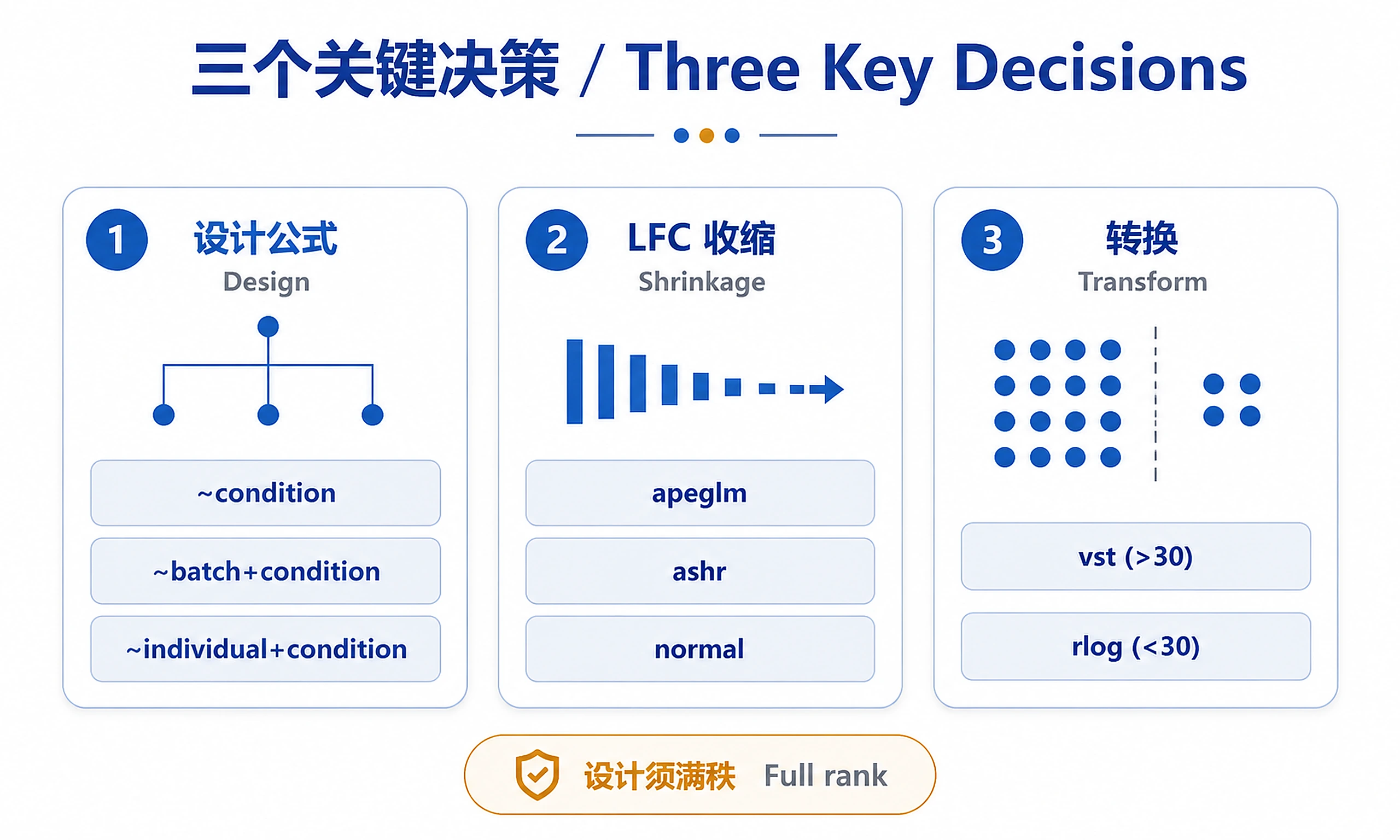
Decision Points
Decision 1: Transformation Method
When: Before creating PCA plots and heatmaps
Options:
- vst(): Use for >30 samples (fast, suitable for large datasets)
- rlog(): Use for <30 samples (better for small samples, slower)
See references/decision-guide.md#decision-point-1 for detailed guidance.
Decision 2: LFC Shrinkage Method
When: Before ranking genes or creating MA/volcano plots
Options:
- apeglm (recommended): Best shrinkage, preserves large LFC
- ashr: Good for large datasets or when apeglm is slow
- normal: Legacy method, not recommended
See references/decision-guide.md#decision-point-2 for detailed guidance.
Decision 3: Design Formula
When: Before creating DESeqDataSet
Options:
- ~ condition: Simple design, no known batch effects
- ~ batch + condition: Known batch effects (requires balanced design)
- ~ individual + condition: Paired samples
- ~ genotype * treatment: Test interactions
Check PCA first - if samples cluster by batch, add batch to design.
See references/decision-guide.md#decision-point-3 for detailed guidance.
Common Issues
| Issue | Solution | Details |
|---|---|---|
| Not seeing verification messages ("✓ Pasilla dataset loaded successfully", "✓ Basic workflow completed successfully!") | You wrote inline code instead of using source(). Stop and use the 3 commands in Standard Workflow section exactly as shown. | See Standard Workflow section |
| "cannot open file" or "No such file" when using absolute paths | Use relative paths ONLY: source("scripts/file.R") not /mnt/knowhow/... or /workspace/.... Skills use relative paths that work in any environment. |
See Standard Workflow section |
"cannot open file" for scripts/load_example_data.R |
Working directory is not the skill root. Use setwd("bulk-rnaseq-counts-to-de-deseq2") or run from correct directory. |
Troubleshooting |
| "trying to use CRAN without setting a mirror" | Set with options(repos = c(CRAN = "https://cloud.r-project.org")) before install.packages() (scripts handle this automatically) |
Troubleshooting |
| "there is no package called 'X'" | Install with BiocManager::install('X') (set CRAN mirror first, or use scripts which handle this) |
Troubleshooting |
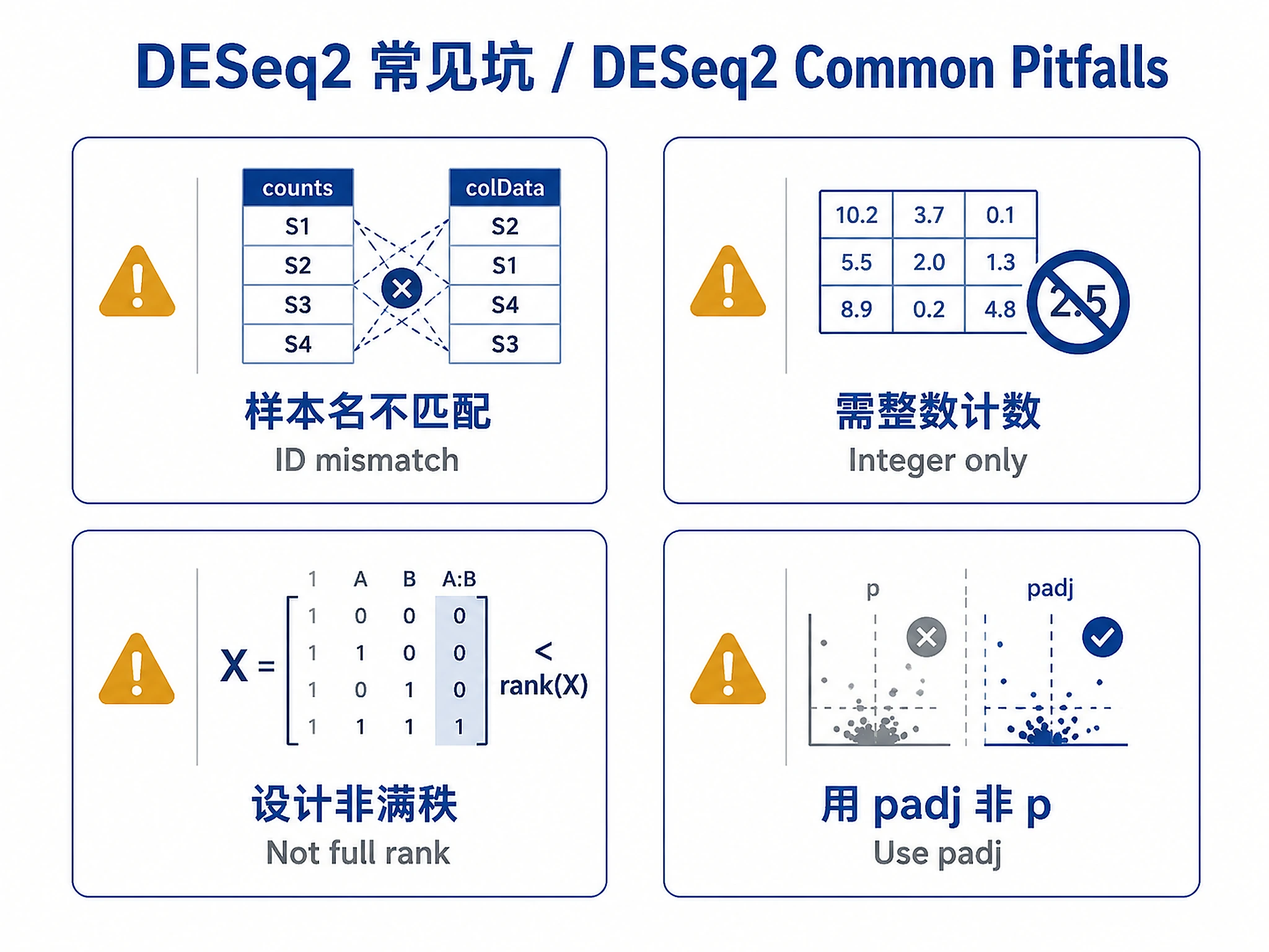
| Sample ID mismatch errors | PREVENTION: Use source("scripts/load_example_data.R"); validate_input_data(counts, coldata) BEFORE creating DESeqDataSet. FIX: Check colnames(counts) vs rownames(coldata) for typos/suffixes |
Troubleshooting |
| Pasilla data sample name mismatch (untreated1 vs untreated1fb) | Use load_pasilla_data() from scripts/load_example_data.R - automatically fixes "fb" suffix issue |
Troubleshooting |
| "design matrix not full rank" | Remove confounded variables or combine into single factor | Troubleshooting |
| "counts should be integers" | Use DESeqDataSetFromTximport() for tximport data |
Troubleshooting |
| "factor levels not in colData" | Check spelling in design formula vs colData columns | Troubleshooting |
| Missing ggplot2/ggprism/ggrepel errors | Install with install.packages(c('ggplot2', 'ggprism', 'ggrepel')) (or use scripts/qc_plots.R which handles installation) |
See Installation section |
| SVG files missing (only PNG generated) | Install svglite: install.packages('svglite'). Note: PNG output is identical quality for analysis (300 DPI). |
See Installation section |
| NA values in padj | Normal - independent filtering removes low-count genes | Troubleshooting |
| No significant genes | Check PCA for batch effects, verify reference level | Troubleshooting |
See references/troubleshooting.md for comprehensive troubleshooting guide.
Best Practices
- 🚨 CRITICAL: Use source() commands from Standard Workflow - DO NOT write inline code - Verify you see success messages: "✓ Pasilla dataset loaded successfully", "✓ Basic workflow completed successfully!" - Scripts handle all package installation, validation, and error checking automatically
- ✅ REQUIRED: Validate sample IDs match between counts and metadata (scripts do this automatically, or use
validate_input_data()) - ✅ REQUIRED: Pre-filter low-count genes before
DESeq()(basic_workflow.R does this) - ✅ REQUIRED: Set reference level explicitly with
relevel()(basic_workflow.R does this) - ✅ REQUIRED: Apply LFC shrinkage for visualization/ranking, use unshrunk for testing (basic_workflow.R does this)
- ✅ Use padj (not pvalue) for significance calling
- ✅ Check QC plots before trusting results (PCA, dispersion, MA) - use
run_all_qc() - ✅ Use vst() for >30 samples, rlog() for <30 samples (qc_plots.R auto-selects)
- ✅ Document design formula and report DESeq2 version
Suggested Next Steps
After completing DESeq2 analysis, you'll typically want to:
1. Filter and Export Results (de-results-to-gene-lists skill)
RECOMMENDED NEXT STEP - Use the de-results-to-gene-lists skill to:
- Filter significant genes (padj < 0.05, |log2FC| > 1)
- Add gene annotations (symbols, descriptions, IDs)
- Export to CSV, Excel, or gene list formats
- Create ranked gene lists for GSEA
Example prompt: "Filter the DESeq2 results to get significant genes with padj < 0.05 and |log2FC| > 1, add gene annotations, and export to CSV and Excel"
Inputs needed: The res and dds objects from this analysis
2. Create Advanced Visualizations (de-results-to-plots skill)
OPTIONAL - This skill already generates basic QC plots (PCA, MA, volcano, dispersion). Use the de-results-to-plots skill for:
- Publication-quality visualizations with advanced customization
- Heatmaps of top differentially expressed genes
- Sample distance matrices
- Expression plots for specific genes of interest
Example prompt: "Create a heatmap of the top 50 significant genes and expression plots for genes FBgn0039155, FBgn0025111"
Inputs needed: The res, dds, and transformed count data from this analysis
3. Functional Enrichment Analysis
After filtering significant genes (using de-results-to-gene-lists):
- pathway-analysis - GO/KEGG enrichment of gene lists
- gsea
- Gene set enrichment on ranked genes
4. Quality Control
If you see issues in QC plots:
- Batch effects in PCA: Re-run with
~ batch + conditiondesign - Poor sample clustering: Check sample metadata for swaps/errors
- High dispersion: May indicate low quality samples
Related Skills
Alternative methods (use instead of this skill):
- edger - Use for small samples (n=2-3) or many contrasts (coming soon)
- limma-voom - Use for normalized data (TPM/FPKM) (coming soon)
References
Detailed documentation:
- references/deseq2-reference.md - Complete code patterns and examples
- references/decision-guide.md - Detailed decision-making guidance
- references/troubleshooting.md - Comprehensive error solutions
Scripts:
- scripts/basic_workflow.R - Complete example workflow
- scripts/qc_plots.R - Quality control functions
- scripts/extract_results.R - Results extraction functions
- scripts/export_results.R - Export functions
- scripts/transformations.R - Transformation functions
Official documentation:
- DESeq2 Bioconductor: http://bioconductor.org/packages/DESeq2
- DESeq2 paper: Love et al. (2014) Genome Biology
License: LGPL (>= 3) (commercial use permitted)
Code preview
scripts/basic_workflow.R
# Basic DESeq2 workflow for differential expression analysis
#
# This script demonstrates the complete DESeq2 workflow using example data.
# For your own data, replace the data loading section with your count matrix and metadata.

library(DESeq2)
library(apeglm)

# =============================================================================
# STEP 1: LOAD DATA
# =============================================================================

# --- OPTION A: Use example dataset (for testing) ---
source("scripts/load_example_data.R")
data <- load_pasilla_data()  # Installs pasilla if needed
counts <- data$counts
coldata <- data$coldata

# Prepare coldata for simple two-group comparison
coldata <- coldata[, "condition", drop = FALSE]  # Keep only condition column

# --- OPTION B: Load your own data (uncomment and modify) ---
# counts <- read.csv("path/to/counts.csv", row.names = 1)
# coldata <- read.csv("path/to/metadata.csv", row.names = 1)
# counts <- as.matrix(counts)  # Ensure counts is a matrix

# --- OPTION C: Use airway dataset (alternative example) ---
# source("scripts/load_example_data.R")
# data <- load_airway_data()
# counts <- data$counts
# coldata <- data$coldata[, "dex", drop = FALSE]
# colnames(coldata) <- "condition"  # Rename for consistency

# =============================================================================
# STEP 2: VALIDATE DATA (CRITICAL - prevents errors downstream)
# =============================================================================

cat("=== Data Validation ===\n")
if (!all(colnames(counts) %in% rownames(coldata))) {
  missing <- setdiff(colnames(counts), rownames(coldata))
  stop("Sample ID mismatch!\n",
       "  Count columns not in metadata: ", paste(head(missing, 5), collapse = ", "))
}

# Reorder coldata to match counts
coldata <- coldata[colnames(counts), , drop = FALSE]

cat("✓ Sample IDs validated\n")
cat("  Dimensions:", nrow(counts), "genes x", ncol(counts), "samples\n")
cat("  Groups:", paste(table(coldata$condition), "samples per group"), "\n\n")

# =============================================================================
# STEP 3: CREATE DESeqDataSet
# =============================================================================

cat("=== Creating DESeqDataSet ===\n")
dds <- DESeqDataSetFromMatrix(
  countData = counts,
  colData = coldata,
  design = ~ condition
)

cat("✓ DESeqDataSet created\n")
cat("  Design: ~ condition\n\n")

# =============================================================================
# STEP 4: PRE-FILTER LOW-COUNT GENES (REQUIRED - improves power)
# =============================================================================

cat("=== Pre-filtering Genes ===\n")
cat("Genes before filtering:", nrow(dds), "\n")

keep <- rowSums(counts(dds)) >= 10
dds <- dds[keep, ]

cat("Genes after filtering:", nrow(dds), "\n")
cat("Genes removed:", sum(!keep), "\n\n")

# =============================================================================
# STEP 5: SET REFERENCE LEVEL (REQUIRED - ensures correct comparison direction)
scripts/batch_correction.R
# DESeq2 with batch effect correction

library(DESeq2)
library(apeglm)

# Example with batch effects
set.seed(42)
n_genes <- 1000
n_samples <- 12

counts <- matrix(rnbinom(n_genes * n_samples, mu = 100, size = 10),
                 nrow = n_genes,
                 dimnames = list(paste0('gene', 1:n_genes),
                                paste0('sample', 1:n_samples)))

coldata <- data.frame(
    condition = factor(rep(c('control', 'treated'), 6)),
    batch = factor(rep(c('batch1', 'batch2', 'batch3'), each = 4)),
    row.names = colnames(counts)
)

# Create DESeqDataSet with batch in design
dds <- DESeqDataSetFromMatrix(countData = counts,
                               colData = coldata,
                               design = ~ batch + condition)

# Pre-filter
keep <- rowSums(counts(dds)) >= 10
dds <- dds[keep,]

# Set reference level
dds$condition <- relevel(dds$condition, ref = 'control')

# Run DESeq2
dds <- DESeq(dds)

# Check available coefficients
cat('Available coefficients:\n')
print(resultsNames(dds))

# Get results for condition effect (controlling for batch)
res <- lfcShrink(dds, coef = 'condition_treated_vs_control', type = 'apeglm')

summary(res)
scripts/export_results.R
# Export DESeq2 results and normalized data
# Functions for saving results tables and transformed counts

library(DESeq2)

#' Export all DESeq2 results to CSV
#'
#' @param res DESeqResults object
#' @param output_file Output file path (CSV)
#'
#' @export
export_results <- function(res, output_file = "deseq2_results.csv") {
    write.csv(as.data.frame(res), file = output_file, row.names = TRUE)
    cat("All results saved to:", output_file, "\n")
    cat("  Total genes:", nrow(res), "\n")
}

#' Export significant genes only
#'
#' @param res DESeqResults object
#' @param padj_threshold Adjusted p-value threshold (default: 0.05)
#' @param lfc_threshold Log2 fold change threshold (default: 0, no filtering)
#' @param output_file Output file path (CSV)
#'
#' @export
export_significant <- function(res, padj_threshold = 0.05, lfc_threshold = 0,
                                output_file = "deseq2_significant.csv") {
    sig <- subset(res, padj < padj_threshold & abs(log2FoldChange) > lfc_threshold)

    write.csv(as.data.frame(sig), file = output_file, row.names = TRUE)

    cat("Significant genes saved to:", output_file, "\n")
    cat("  Threshold: padj <", padj_threshold, ", |log2FC| >", lfc_threshold, "\n")
    cat("  Total significant:", nrow(sig), "\n")
    cat("    Upregulated:", sum(sig$log2FoldChange > 0, na.rm = TRUE), "\n")
    cat("    Downregulated:", sum(sig$log2FoldChange < 0, na.rm = TRUE), "\n")
}

#' Export normalized counts
#'
#' @param dds DESeqDataSet object (after DESeq())
#' @param output_file Output file path (CSV)
#'
#' @export
export_normalized_counts <- function(dds, output_file = "normalized_counts.csv") {
    norm_counts <- counts(dds, normalized = TRUE)
    write.csv(norm_counts, file = output_file, row.names = TRUE)
    cat("Normalized counts saved to:", output_file, "\n")
}

#' Export variance-stabilized counts
#'
#' @param dds DESeqDataSet object (after DESeq())
#' @param output_file Output file path (CSV)
#' @param use_vst Use VST (TRUE) or rlog (FALSE)
#'
#' @export
export_transformed_counts <- function(dds, output_file = "vst_transformed.csv",
                                      use_vst = TRUE) {
    if (use_vst) {
        transformed <- vst(dds, blind = FALSE)
        cat("Using VST transformation\n")
    } else {
        transformed <- rlog(dds, blind = FALSE)
        cat("Using rlog transformation\n")
        # Update filename if using rlog
        if (output_file == "vst_transformed.csv") {
            output_file <- "rlog_transformed.csv"
        }
    }

    write.csv(assay(transformed), file = output_file, row.names = TRUE)
    cat("Transformed counts saved to:", output_file, "\n")
}

#' Export top genes by significance or fold change
#'
#' @param res DESeqResults object
#' @param n Number of top genes to export (default: 100)
#' @param order_by Order by 'padj' or 'lfc' (default: 'padj')
Companion files
| Type | Path | Bytes |
|---|---|---|
| Markdown | references/comprehensive-reference.md | 8,999 |
| Markdown | references/decision-guide.md | 8,561 |
| Markdown | references/troubleshooting.md | 8,735 |
| Markdown | references/usage-guide.md | 2,122 |
| R | scripts/basic_workflow.R | 5,748 |
| R | scripts/batch_correction.R | 1,182 |
| R | scripts/export_results.R | 6,787 |
| R | scripts/extract_results.R | 7,731 |
| R | scripts/load_example_data.R | 8,290 |
| R | scripts/multi_condition.R | 1,551 |
| R | scripts/qc_plots.R | 14,150 |
| R | scripts/transformations.R | 6,252 |
| Markdown | SKILL.md | 24,398 |
| JSON | skill.meta.json | 2,608 |