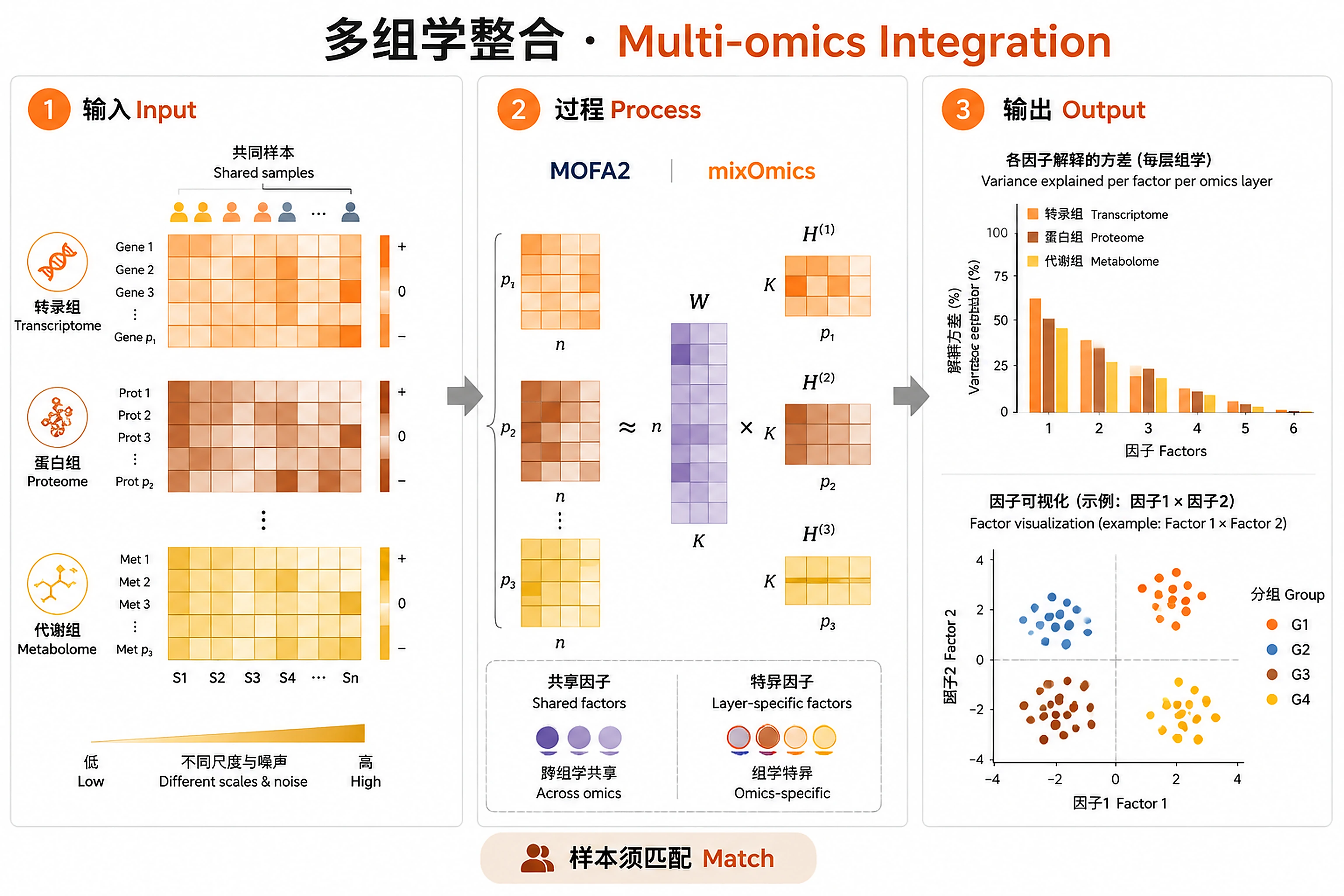
Multi-omics Integration
Integrate 2+ omics into interpretable latent factors.
Overview
Problem. Each layer has its own scale and noise; naive merging distorts.
Learning goals
- A few latent factors explain cross-layer variance
- Shared vs layer-specific factors
Figures
Tutorial
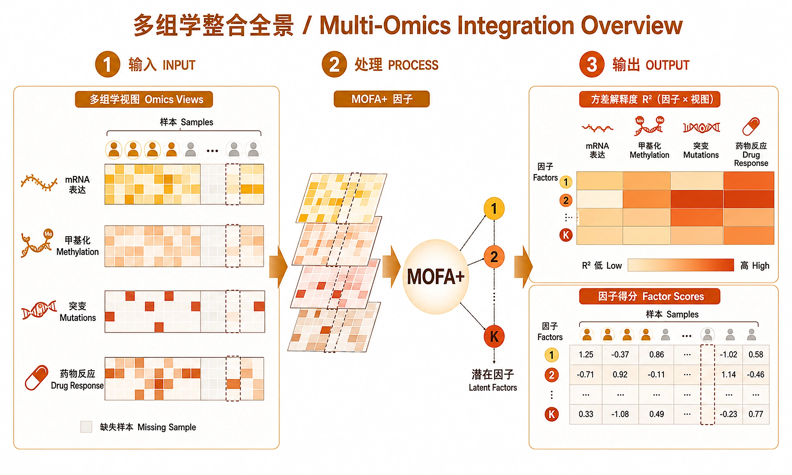
Identify latent factors driving variation across 2+ omics layers using MOFA+ (Multi-Omics Factor Analysis). Decomposes multi-omics data into interpretable factors, each capturing shared or view-specific biological signal. Handles missing data across views natively.
When to Use This Skill
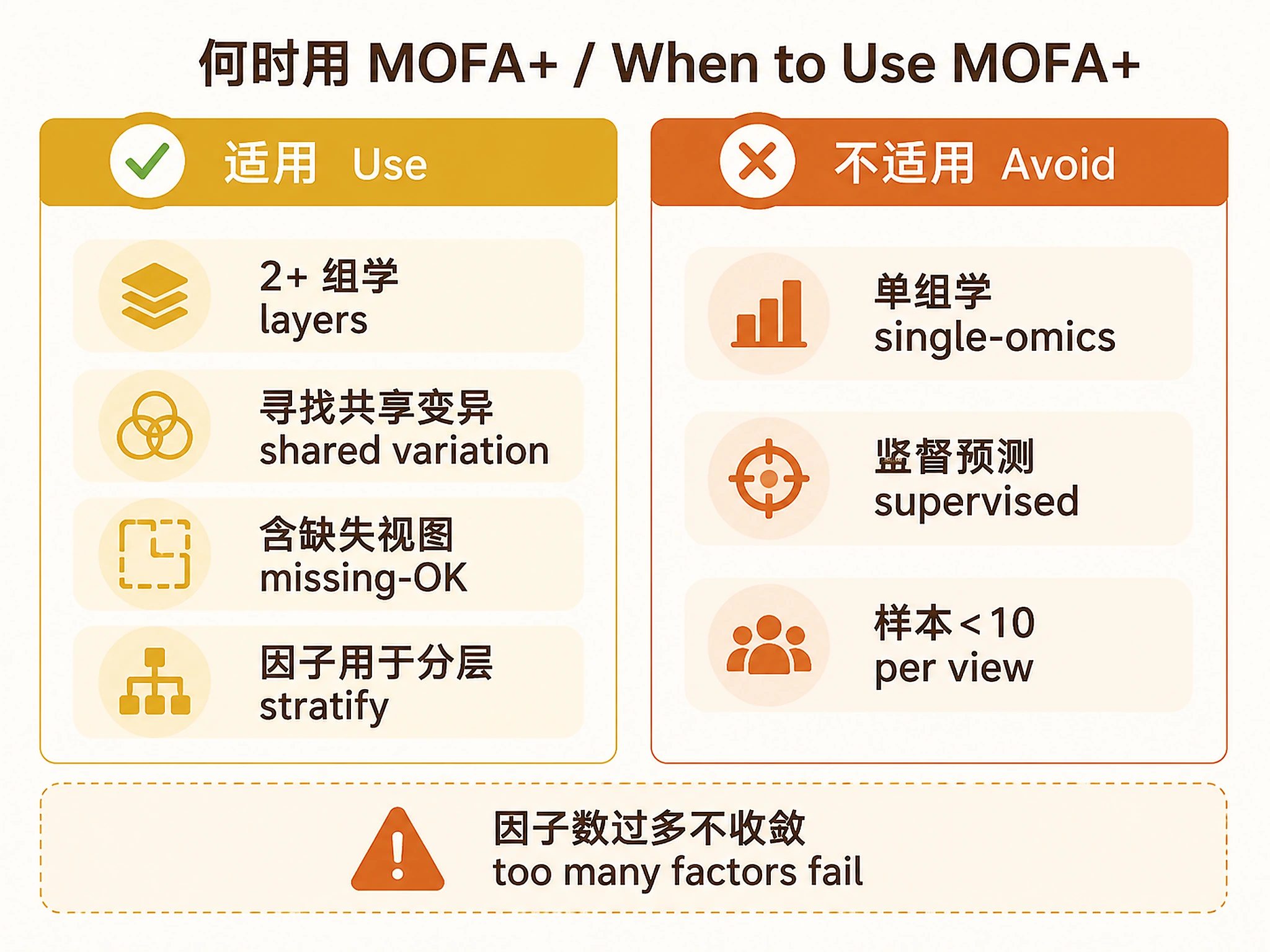
Use when you:
- ✅ Have 2+ omics layers measured on overlapping samples (RNA-seq + proteomics, methylation + mutations, etc.)
- ✅ Want to find shared sources of variation across omics (not just per-omics analysis)
- ✅ Need to identify which omics layers contribute to each source of variation
- ✅ Have incomplete data (not all samples measured in all views) — MOFA handles this
- ✅ Want factor scores for downstream patient stratification or survival analysis
Don't use for:
- ❌ Single omics data (use
bulk-rnaseq-counts-to-de-deseq2orbulk-omics-clustering) - ❌ Supervised prediction (use
lasso-biomarker-panelinstead) - ❌ Single-cell multi-modal (MOFA2 supports it, but consider
scrna-trajectory-inference) - ❌ Fewer than 10 samples per view
Runtime: ~5-8 minutes total (CLL example). First run adds ~1-3 min for Python environment setup.
Installation
# Bioconductor packages
if (!requireNamespace("BiocManager", quietly = TRUE)) install.packages("BiocManager")
BiocManager::install(c("MOFA2", "MOFAdata", "ComplexHeatmap"))

# CRAN packages
install.packages(c("ggprism", "circlize", "reshape2", "RColorBrewer"))
| Package | Version | License | Commercial Use | Installation |
|---|---|---|---|---|
| MOFA2 | ≥1.12.0 | LGPL (≥3) | ✅ Permitted | BiocManager::install("MOFA2") |
| MOFAdata | ≥1.8.0 | Artistic-2.0 | ✅ Permitted | BiocManager::install("MOFAdata") (example data) |
| ComplexHeatmap | ≥2.18.0 | MIT | ✅ Permitted | BiocManager::install("ComplexHeatmap") |
| ggprism | ≥1.0.3 | GPL (≥3) | ✅ Permitted | install.packages("ggprism") |
| circlize | ≥0.4.15 | MIT | ✅ Permitted | install.packages("circlize") |
| reshape2 | ≥1.4.4 | MIT | ✅ Permitted | install.packages("reshape2") |
| RColorBrewer | ≥1.1 | Apache-2.0 | ✅ Permitted | install.packages("RColorBrewer") |
| rmarkdown | ≥2.25 | GPL-3 | ✅ Permitted | install.packages("rmarkdown") (optional, PDF) |
Inputs
- Multi-omics data: Named list of matrices (features × samples), one per omics view
- Minimum 2 views, any combination of omics types
- Samples as columns, features as rows
- Missing samples across views OK (MOFA handles incomplete overlap)
- Sample metadata (optional): CSV/TSV with sample IDs + clinical variables (for factor-trait associations)
- Supported formats: R matrices, CSV/TSV files, or MultiAssayExperiment
Outputs
Analysis objects (RDS):
mofa_model.rds— Complete trained MOFA model for downstream use- Load with:
model <- readRDS('mofa_results/mofa_model.rds') - Required for:
bulk-omics-clustering(factor-based clustering),lasso-biomarker-panel(feature selection)
CSV results:
factor_values.csv— Sample factor scores (samples × factors)weights_*.csv— Feature weights per view (features × factors)variance_explained_per_factor.csv— R² per factor per viewvariance_explained_total.csv— Total R² per viewtop_features_per_factor.csv— Top 20 features per factor per view
Visualizations (PNG + SVG):
mofa_variance_per_factor— Heatmap: R² per factor per view (signature MOFA plot)mofa_total_variance— Bar chart: total R² per viewmofa_factor_scatter— Scatter: Factor 1 vs 2 colored by clinical variablemofa_factor_correlation— Tile: factor-factor correlationsmofa_top_weights— Faceted bar: top feature weights per factormofa_factor_heatmap— ComplexHeatmap: factors × samples with annotationsmofa_factor_clinical— Box plots: factor values by clinical groups
Reports:
analysis_report.md— Markdown summary with methods, results, referencesanalysis_report.pdf— PDF report with embedded figures (requires rmarkdown + LaTeX)
Clarification Questions
- Input Files (ASK THIS FIRST): - Do you have multi-omics data matrices to integrate? - Expected: Named list of matrices (features × samples), or CSV files per omics view - Or use example data? CLL blood cancer dataset (200 patients: mRNA, methylation, mutations, drug response)
🚨 IF EXAMPLE DATA SELECTED: Skip questions 3-4. Proceed directly to Step 1.
-
Analysis Options:
- (If using example data) Number of factors:
- a) 15 factors — standard analysis (recommended)
- b) 5 factors — quick demo (~2 min faster)
- (If using own data) Number of factors:
- a) 15 (recommended starting point)
- b) Custom number
-
(Own data only) Data types per view:
- Which omics types? (RNA-seq, proteomics, methylation, mutations, metabolomics, drug response, other)
- Are any views binary (0/1)? MOFA uses Bernoulli likelihood for binary data.
-
(Own data only) Sample metadata:
- Do you have a sample metadata file (CSV/TSV) with clinical variables?
- Variables for factor-trait associations (e.g., disease status, treatment, subtype)?
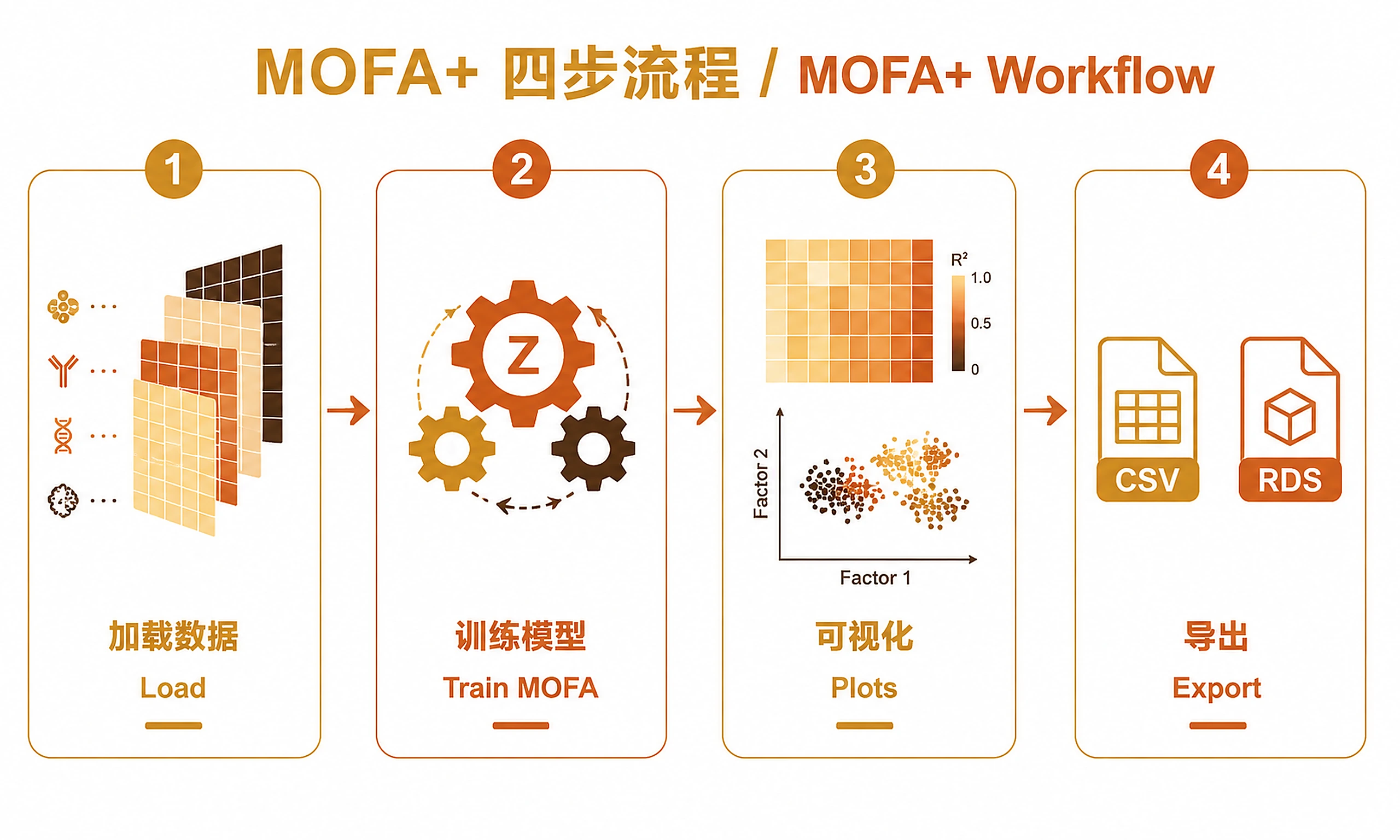
Standard Workflow
🚨 MANDATORY: USE SCRIPTS EXACTLY AS SHOWN - DO NOT WRITE INLINE CODE 🚨
Step 1 - Load data:
# For CLL example data:
source("scripts/load_example_data.R")
cll <- load_cll_data()

# For user data:
# source("scripts/load_example_data.R")
# cll <- load_user_data(
#   file_paths = list(RNA = "rna.csv", Protein = "protein.csv"),
#   metadata_path = "metadata.csv"
# )
✅ VERIFICATION: "✓ Data loaded successfully!" with per-view dimensions
Step 2 - Run MOFA analysis:
source("scripts/mofa_workflow.R")
model <- run_mofa_analysis(
    data_list = cll$data,
    metadata = cll$metadata,
    n_factors = 15,
    output_dir = "mofa_results"
)
DO NOT write inline MOFA code. Just call run_mofa_analysis().
⏱️ Takes ~2-5 min (+ ~1-3 min extra on first run for Python environment setup via basilisk).
✅ VERIFICATION: "✓ MOFA model trained successfully!" with variance explained summary
Step 3 - Generate visualizations:
source("scripts/mofa_plots.R")
generate_all_plots(model, output_dir = "mofa_results")
DO NOT write inline plotting code (ggsave, ggplot, Heatmap, etc.). Just use the script.
The script handles PNG + SVG export with graceful fallback for SVG dependencies.
✅ VERIFICATION: "✓ All plots generated successfully!" with file count
Step 4 - Export results:
source("scripts/export_results.R")
export_all(model, output_dir = "mofa_results")
DO NOT write custom export code. Use export_all().
✅ VERIFICATION: "=== Export Complete ===" with file list
⚠️ CRITICAL - DO NOT:
- ❌ Write inline MOFA code → STOP: Use
run_mofa_analysis() - ❌ Write inline plotting code (ggsave, ggplot, Heatmap, etc.) → STOP: Use
generate_all_plots() - ❌ Write custom export code → STOP: Use
export_all() - ❌ Try to install basilisk/reticulate manually → MOFA2 handles Python automatically
⚠️ IF SCRIPTS FAIL - Script Failure Hierarchy:
- Fix and Retry (90%) — Install missing package, re-run script
- Modify Script (5%) — Edit the script file itself, document changes
- Use as Reference (4%) — Read script, adapt approach, cite source
- Write from Scratch (1%) — Only if genuinely impossible, explain why
NEVER skip directly to writing inline code without trying the script first.
Common Issues
| Error | Cause | Solution |
|---|---|---|
| basilisk Python env setup slow | First-time setup of Python backend | Normal — wait 1-3 minutes. Only happens once per R installation. |
run_mofa hangs at "Training model..." |
Model training in progress | Normal — wait 2-5 min. Training is compute-intensive. |
Error in py_call_impl: Python error |
basilisk environment issue | Restart R session, retry. If persistent: BiocManager::install("MOFA2", force = TRUE) |
| Metadata download failed | EBI FTP blocked or offline | Normal fallback. Analysis runs without trait plots. Metadata is optional. |
| "No convergence" | Too many factors or too few samples | Reduce n_factors (try 5-10). Ensure ≥10 samples. |
| SVG export failed | Missing svglite/cairo | Normal. PNG always generated. generate_all_plots() handles fallback automatically. |
| Memory error | Dataset too large | Filter features to top 5,000 most variable per view before MOFA. |
Interpretation Guide
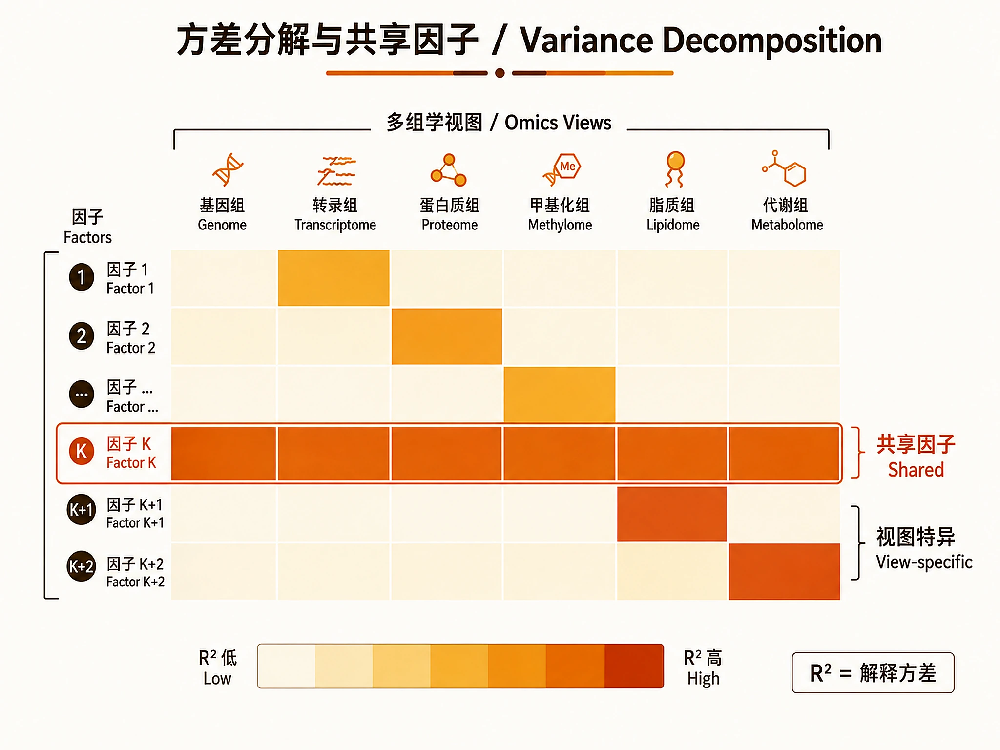
Variance Decomposition (Key MOFA Output)
- High R² in one view: Factor captures view-specific variation
- High R² across views: Factor captures shared cross-omics signal (most interesting)
- Low total R²: MOFA explains little variation in that view — consider adding features or views
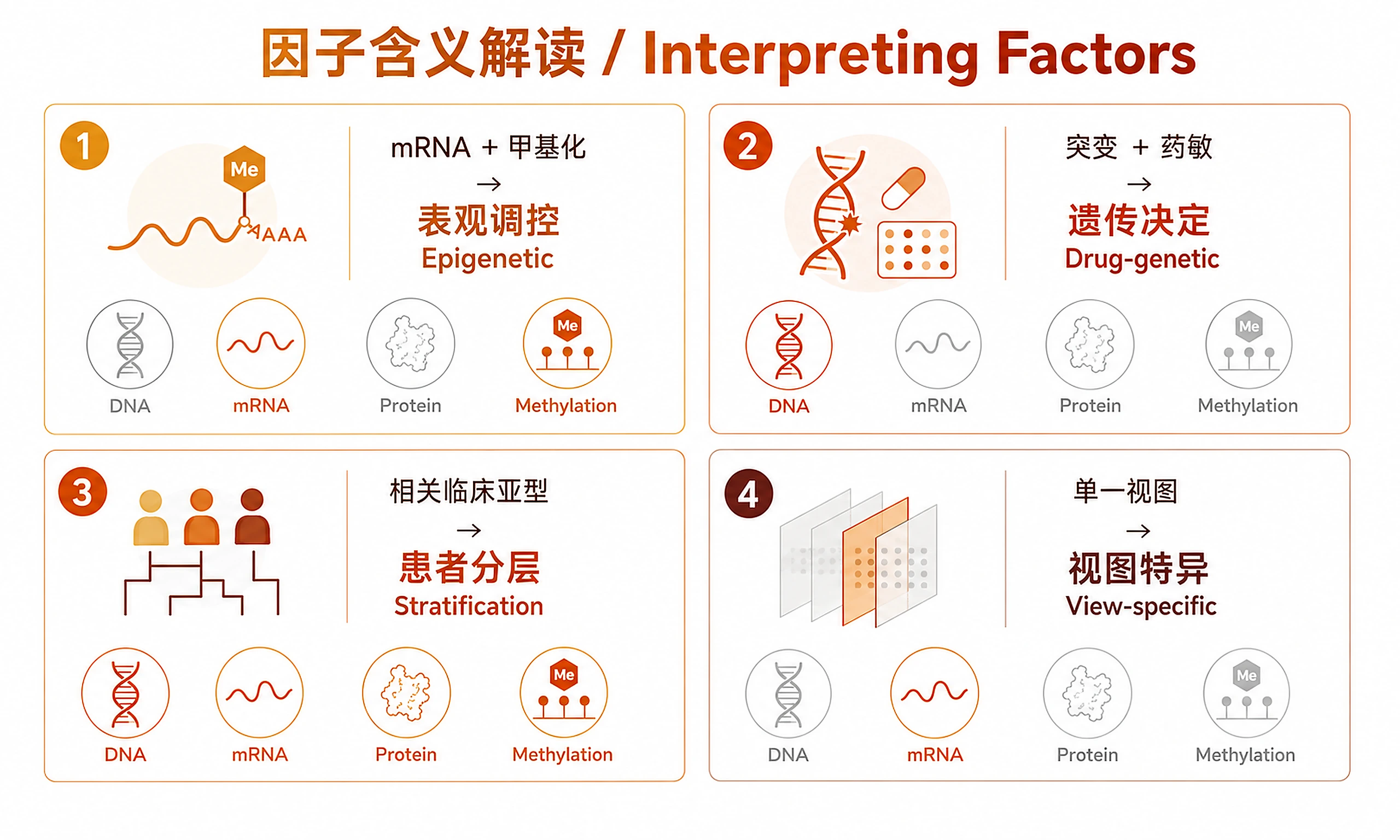
Factor Interpretation
| Pattern | Meaning |
|---|---|
| Factor active in mRNA + methylation | Epigenetic regulation of transcription |
| Factor active in mutations + drug response | Genetic determinants of drug sensitivity |
| Factor correlates with clinical subtype | Biologically meaningful patient stratification |
| Factor active in only one view | View-specific technical or biological variation |
See: references/mofa-interpretation-guide.md for detailed downstream analysis.
Suggested Next Steps
After running MOFA:
- Patient stratification: Use
bulk-omics-clusteringon factor scores to define molecular subtypes - Biomarker discovery: Use
lasso-biomarker-panelon top-weighted features per factor - Pathway enrichment: Use
functional-enrichment-from-degson top mRNA features per factor - Network analysis: Use
coexpression-networkon factor-associated genes - Survival analysis: Use
survival-analysis-clinicalwith factor scores as covariates
Related Skills
| Skill | Relationship |
|---|---|
bulk-omics-clustering |
Downstream: cluster on MOFA factor scores |
lasso-biomarker-panel |
Downstream: select biomarkers from top factor features |
disease-progression-longitudinal |
Complementary: trajectory analysis on factor scores |
coexpression-network |
Downstream: network analysis on factor-associated genes |
functional-enrichment-from-degs |
Downstream: pathway enrichment on top factor features |
bulk-rnaseq-counts-to-de-deseq2 |
Upstream: generate DE results as one omics view |
References
- Argelaguet R, et al. (2020) MOFA+: a statistical framework for comprehensive integration of multi-modal single-cell data. Genome Biology 21:111.
- Argelaguet R, et al. (2018) Multi-Omics Factor Analysis—a framework for unsupervised integration of multi-omics data sets. Molecular Systems Biology 14:e8124.
- Dietrich S, et al. (2018) Drug-perturbation-based stratification of blood cancer. Journal of Clinical Investigation 128(1):427-445.
Code preview
scripts/export_results.R
# =============================================================================
# Export MOFA+ Analysis Results
# =============================================================================
# Exports factor values, feature weights, variance explained, and analysis
# objects. Generates markdown summary report and optional PDF report.
# =============================================================================

options(repos = c(CRAN = "https://cloud.r-project.org"))

.install_if_missing <- function(pkg, bioc = FALSE) {
    if (!requireNamespace(pkg, quietly = TRUE)) {
        cat("Installing", pkg, "...\n")
        if (bioc) {
            if (!requireNamespace("BiocManager", quietly = TRUE))
                install.packages("BiocManager")
            BiocManager::install(pkg, ask = FALSE, update = FALSE)
        } else {
            install.packages(pkg)
        }
    }
}

#' Export all MOFA analysis results
#'
#' @param model Trained MOFA model object
#' @param output_dir Directory for output files
export_all <- function(model, output_dir = "mofa_results") {

    cat("\n=== Exporting MOFA Analysis Results ===\n\n")

    .install_if_missing("MOFA2", bioc = TRUE)
    .install_if_missing("reshape2")
    library(MOFA2)

    if (!dir.exists(output_dir)) {
        dir.create(output_dir, recursive = TRUE)
    }

    # -------------------------------------------------------------------------
    # 1. Factor values (samples x factors)
    # -------------------------------------------------------------------------
    cat("1. Exporting factor values...\n")
    factors_df <- get_factors(model, as.data.frame = TRUE)
    factors_wide <- reshape2::dcast(factors_df, sample ~ factor, value.var = "value")
    write.csv(factors_wide, file.path(output_dir, "factor_values.csv"), row.names = FALSE)
    cat(sprintf("   %d samples x %d factors\n", nrow(factors_wide), ncol(factors_wide) - 1))
    cat(sprintf("   Saved: %s\n\n", file.path(output_dir, "factor_values.csv")))

    # -------------------------------------------------------------------------
    # 2. Feature weights per view
    # -------------------------------------------------------------------------
    cat("2. Exporting feature weights per view...\n")
    weights_df <- get_weights(model, as.data.frame = TRUE)
    views <- unique(weights_df$view)
    for (v in views) {
        w_sub <- weights_df[weights_df$view == v, ]
        w_wide <- reshape2::dcast(w_sub, feature ~ factor, value.var = "value")
        fname <- sprintf("weights_%s.csv", gsub("[^a-zA-Z0-9]", "_", tolower(v)))
        write.csv(w_wide, file.path(output_dir, fname), row.names = FALSE)
        cat(sprintf("   %s: %d features x %d factors -> %s\n",
                    v, nrow(w_wide), ncol(w_wide) - 1, fname))
    }
    cat("\n")

    # -------------------------------------------------------------------------
    # 3. Variance explained
    # -------------------------------------------------------------------------
    cat("3. Exporting variance explained...\n")
    r2 <- get_variance_explained(model)
    r2_per_factor <- r2$r2_per_factor[[1]]
    r2_total <- r2$r2_total[[1]]

    # Per-factor per-view
    r2_df <- as.data.frame(r2_per_factor)
    r2_df$Factor <- rownames(r2_df)
    write.csv(r2_df, file.path(output_dir, "variance_explained_per_factor.csv"),
              row.names = FALSE)

    # Total per view
    total_df <- data.frame(View = names(r2_total), Total_R2 = as.numeric(r2_total))
scripts/load_example_data.R
# =============================================================================
# Load Example Data for MOFA+ Multi-Omics Integration
# =============================================================================
# Loads the CLL (Chronic Lymphocytic Leukemia) multi-omics dataset
# from the MOFAdata package. 200 patients, 4 omics layers:
#   - Drugs: drug response (310 features)
#   - Methylation: DNA methylation (4248 features)
#   - mRNA: gene expression (5000 features)
#   - Mutations: somatic mutations (69 features, binary)
#
# Also downloads sample metadata from EBI for clinical annotations.
# =============================================================================

options(repos = c(CRAN = "https://cloud.r-project.org"))

.install_if_missing <- function(pkg, bioc = FALSE) {
    if (!requireNamespace(pkg, quietly = TRUE)) {
        cat("Installing", pkg, "...\n")
        if (bioc) {
            if (!requireNamespace("BiocManager", quietly = TRUE))
                install.packages("BiocManager")
            BiocManager::install(pkg, ask = FALSE, update = FALSE)
        } else {
            install.packages(pkg)
        }
    }
}

#' Load CLL multi-omics example data
#'
#' @return list with components:
#'   - data: named list of 4 matrices (Drugs, Methylation, mRNA, Mutations)
#'   - metadata: data.frame of sample annotations (or NULL if download fails)
load_cll_data <- function() {
    cat("\n=== Loading CLL Multi-Omics Example Data ===\n\n")

    # --- Install/load MOFAdata ---
    .install_if_missing("MOFAdata", bioc = TRUE)
    library(MOFAdata)

    # --- Load CLL dataset ---
    cat("Loading CLL multi-omics data (200 patients, 4 omics layers)...\n")
    utils::data("CLL_data", package = "MOFAdata", envir = environment())

    # Validate structure
    stopifnot(is.list(CLL_data))
    stopifnot(length(CLL_data) >= 4)

    # --- Print per-view summary ---
    cat("\nDataset overview:\n")
    all_samples <- unique(unlist(lapply(CLL_data, colnames)))
    cat(sprintf("  Total unique samples: %d\n", length(all_samples)))
    cat("\n  View summaries:\n")
    for (view_name in names(CLL_data)) {
        mat <- CLL_data[[view_name]]
        n_feat <- nrow(mat)
        n_samp <- ncol(mat)
        pct_missing <- round((1 - n_samp / length(all_samples)) * 100, 1)
        cat(sprintf("    %-15s %5d features x %3d samples (%4.1f%% samples missing)\n",
                    view_name, n_feat, n_samp, pct_missing))
    }

    # --- Sample overlap ---
    sample_lists <- lapply(CLL_data, colnames)
    shared <- Reduce(intersect, sample_lists)
    cat(sprintf("\n  Samples with ALL 4 views: %d / %d (%.0f%%)\n",
                length(shared), length(all_samples),
                100 * length(shared) / length(all_samples)))

    # --- Download sample metadata ---
    metadata <- .download_cll_metadata()

    cat("\n✓ Data loaded successfully!\n\n")
    return(list(data = CLL_data, metadata = metadata))
}

#' Download CLL sample metadata from EBI
#' @return data.frame or NULL if download fails
.download_cll_metadata <- function() {
    cat("\nDownloading sample metadata...\n")
scripts/mofa_plots.R
# =============================================================================
# MOFA+ Visualization: Publication-Quality Plots
# =============================================================================
# Generates 7 plots using ggprism::theme_prism() and ComplexHeatmap.
# All plots saved as PNG + SVG with graceful fallback.
# =============================================================================

options(repos = c(CRAN = "https://cloud.r-project.org"))

.install_if_missing <- function(pkg, bioc = FALSE) {
    if (!requireNamespace(pkg, quietly = TRUE)) {
        cat("Installing", pkg, "...\n")
        if (bioc) {
            if (!requireNamespace("BiocManager", quietly = TRUE))
                install.packages("BiocManager")
            BiocManager::install(pkg, ask = FALSE, update = FALSE)
        } else {
            install.packages(pkg)
        }
    }
}

# --- Load required packages ---
.load_plot_packages <- function() {
    .install_if_missing("ggplot2")
    .install_if_missing("ggprism")
    .install_if_missing("reshape2")
    .install_if_missing("RColorBrewer")
    .install_if_missing("ComplexHeatmap", bioc = TRUE)
    .install_if_missing("circlize")
    .install_if_missing("MOFA2", bioc = TRUE)

    library(ggplot2)
    library(ggprism)
    library(reshape2)
    library(RColorBrewer)
    library(ComplexHeatmap)
    library(circlize)
    library(MOFA2)
    library(grid)
}

# --- PNG + SVG save helper ---
.save_plot <- function(plot_obj, base_name, output_dir, width = 8, height = 6, dpi = 300) {
    png_path <- file.path(output_dir, paste0(base_name, ".png"))
    svg_path <- file.path(output_dir, paste0(base_name, ".svg"))

    # Always save PNG
    ggsave(png_path, plot = plot_obj, width = width, height = height, dpi = dpi, device = "png")
    cat(sprintf("   Saved: %s\n", png_path))

    # Try SVG with fallback
    tryCatch({
        ggsave(svg_path, plot = plot_obj, width = width, height = height, device = "svg")
        cat(sprintf("   Saved: %s\n", svg_path))
    }, error = function(e) {
        tryCatch({
            svg(svg_path, width = width, height = height)
            print(plot_obj)
            dev.off()
            cat(sprintf("   Saved: %s\n", svg_path))
        }, error = function(e2) {
            cat("   (SVG export failed)\n")
        })
    })
}

# --- ComplexHeatmap save helper ---
.save_heatmap <- function(ht, base_name, output_dir, width = 10, height = 8) {
    png_path <- file.path(output_dir, paste0(base_name, ".png"))
    svg_path <- file.path(output_dir, paste0(base_name, ".svg"))

    # PNG
    png(png_path, width = width, height = height, units = "in", res = 300)
    draw(ht)
    dev.off()
    cat(sprintf("   Saved: %s\n", png_path))

    # SVG
    tryCatch({
Companion files
| Type | Path | Bytes |
|---|---|---|
| Markdown | references/mofa-interpretation-guide.md | 4,597 |
| R | scripts/export_results.R | 13,207 |
| R | scripts/load_example_data.R | 6,447 |
| R | scripts/mofa_plots.R | 18,418 |
| R | scripts/mofa_workflow.R | 6,349 |
| Markdown | SKILL.md | 11,142 |
| JSON | skill.meta.json | 1,540 |