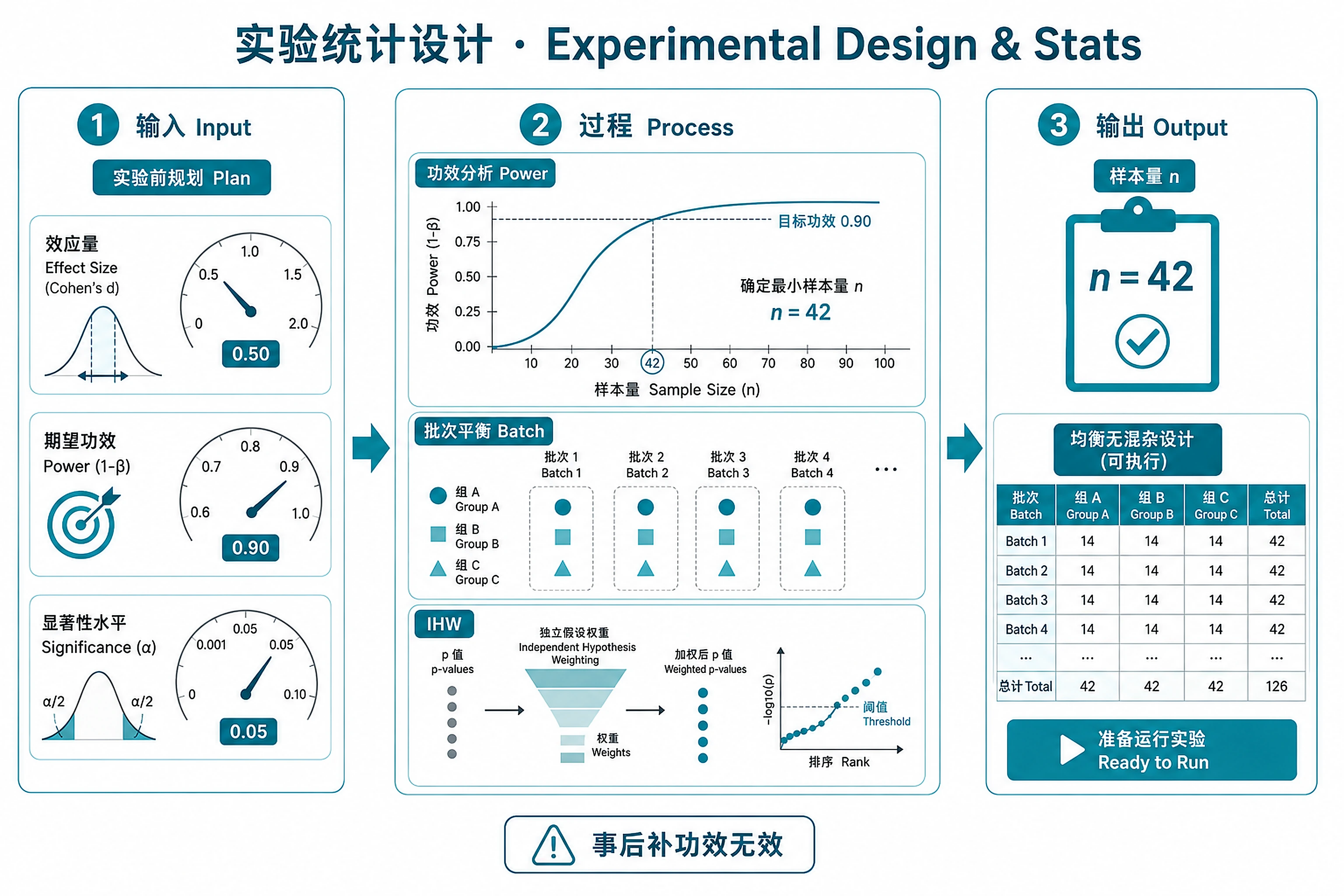
Experimental Design & Stats
Power, sample size, batch balance — before you run.
Overview
Problem. How many samples; how to avoid batch confounding?
Learning goals
- Do the stats before, not after
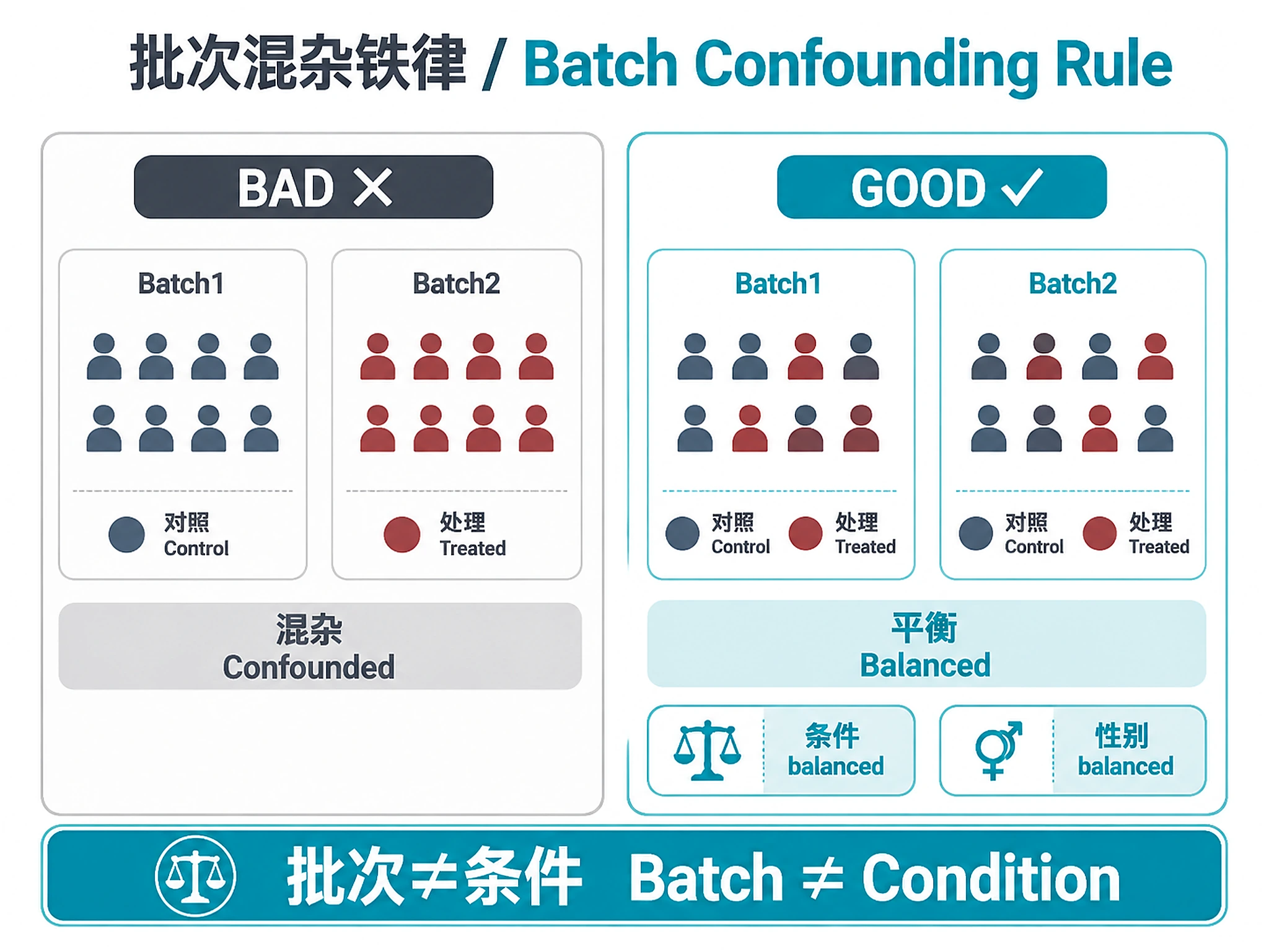
- Batch–group confounding is the top killer
Figures
Tutorial
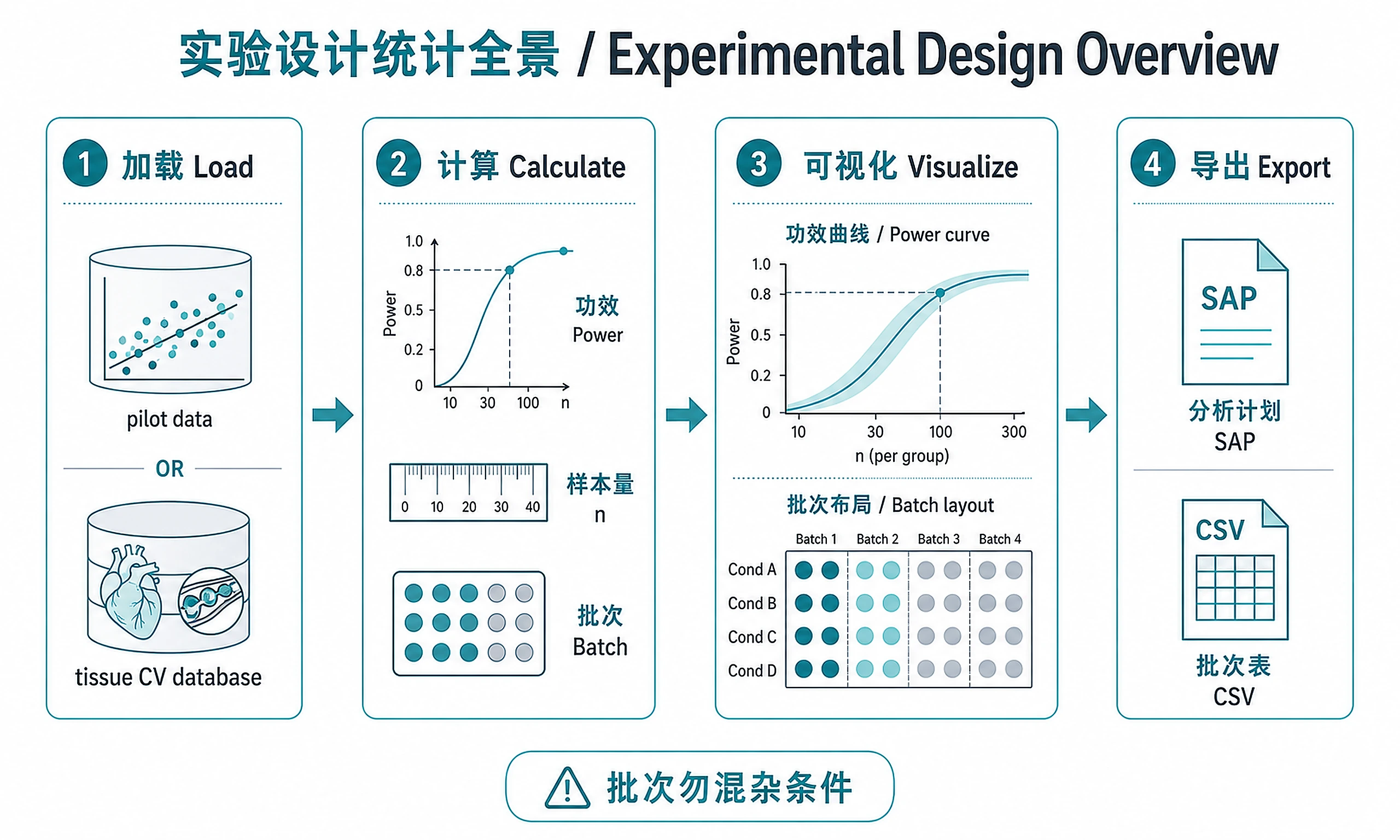
Comprehensive workflow for statistical experimental design in genomics, from power analysis and sample size determination to batch-balanced experimental layouts and multiple testing strategy.
When to Use This Skill
Use this skill when you need to:
- ✅ Plan new experiments
- Design from scratch with statistical rigor
- ✅ Justify sample sizes
- Calculate required replicates for grant proposals
- ✅ Perform power analysis
- Determine statistical power for proposed designs
- ✅ Design batch layouts
- Create balanced assignments preventing confounding
- ✅ Optimize budgets
- Balance sequencing depth vs. number of replicates
- ✅ Select correction methods
- Choose appropriate multiple testing approaches
Don't use this skill for:
- ❌ Post-experiment analysis → Use appropriate DE analysis skills
- ❌ Simple two-sample comparisons with fixed n → Use power calculators directly
Key Concept: Proper experimental design is the foundation of reproducible science. Good design prevents confounding, maximizes statistical power, and ensures results are interpretable.
Installation
Required Software
| Software | Version | License | Commercial Use | Installation |
|---|---|---|---|---|
| DESeq2 | ≥1.30.0 | LGPL (≥3) | ✅ Permitted | BiocManager::install('DESeq2') |
| RNASeqPower | ≥1.30.0 | LGPL | ✅ Permitted | BiocManager::install('RNASeqPower') |
| ssizeRNA | ≥1.3.2 | GPL-2 | ✅ Permitted | BiocManager::install('ssizeRNA') |
| powsimR | ≥1.2.3 | GPL-3 | ✅ Permitted | BiocManager::install('powsimR') |
| IHW | ≥1.18.0 | Artistic-2.0 | ✅ Permitted | BiocManager::install('IHW') |
| osat | ≥1.38.0 | Artistic-2.0 | ✅ Permitted | install.packages('osat') |
| ggplot2 | ≥3.3.0 | MIT | ✅ Permitted | install.packages('ggplot2') |
| ggprism | ≥1.0.3 | GPL-3 | ✅ Permitted | install.packages('ggprism') |
| jsonlite | ≥1.7.0 | MIT | ✅ Permitted | install.packages('jsonlite') |
| pasilla | ≥1.18.0 | Artistic-2.0 | ✅ Permitted | BiocManager::install('pasilla') |
Optional (for example data):
- pasilla - Example RNA-seq pilot data for testing
Quick install:
if (!requireNamespace("BiocManager", quietly = TRUE))
    install.packages("BiocManager")

BiocManager::install(c("DESeq2", "RNASeqPower", "ssizeRNA", "powsimR", "IHW", "pasilla"))
install.packages(c("osat", "ggplot2", "ggprism", "jsonlite"))
License Compliance: All packages use LGPL, GPL, Artistic-2.0, or MIT licenses that permit commercial use in AI agent applications.
Full installation instructions and version details: references/software_requirements.md
Inputs
Required:
- Experimental design info: Assay type, n conditions, sample relationship, planned n
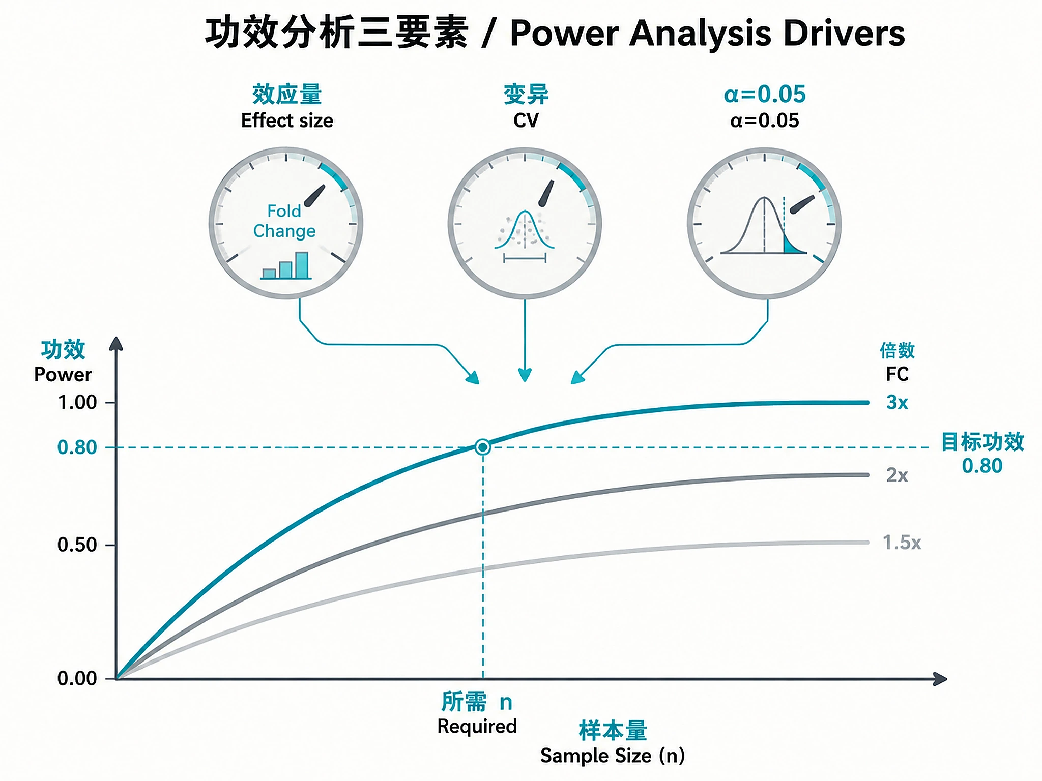
- Effect size expectations: Target fold change, variability (CV or pilot data)
- Statistical requirements: Target power (0.80/0.90), α (0.05), multiple testing preference
Optional:
- Practical constraints: Budget, sample availability, batch structure, sequencing depth, covariates
Detailed input requirements: references/experimental_design_best_practices.md#input-requirements
Outputs
Power and sample size:
power_analysis_results.csv- Power calculations for scenariossample_size_recommendation.txt- Required n with justificationpower_vs_n_curve.png+.svg- Power relationship visualizations
Batch design:
batch_layout_for_lab.csv- Lab-ready sample-to-batch assignmentsbatch_design_validation.txt- Confounding check resultsbatch_design_plot.png+.svg- Visual layout
Documentation:
statistical_analysis_plan.md- Complete pre-registration planlab_protocol_checklist.md- Step-by-step processing guidedesign_parameters.json- All parameters (human-readable)
Analysis objects (RDS) - For downstream use:
batch_design.rds- Complete batch design object- Load with:
batch_design <- readRDS('batch_design.rds') - Required for: Batch effect correction workflows
design_parameters.rds- Complete design parameters- Load with:
design_params <- readRDS('design_parameters.rds') - Required for: Analysis validation, replication studies
Clarification Questions
Before starting, gather the following information:
1. Input Files (ASK THIS FIRST):
- Do you have pilot data or existing results files to inform the experimental design?
- If uploaded: Are these pilot data files (DESeq2 objects, count matrices) you'd like to use for power calculations?
- Expected formats: RDS (DESeqDataSet), CSV/TSV (count matrices)
- Or use literature-based estimates? We can use tissue-specific variability values from published data (references/cv_tissue_database.csv).
2. Assay Type
- Bulk RNA-seq, scRNA-seq, ATAC-seq, ChIP-seq, Methylation, Proteomics, or Other
3. Experimental Structure
- Conditions: 2 (case-control), 3+ (multi-group), or factorial design?
- Planned n: Replicates per condition (or "unknown")
- Sample type: Independent, paired, or repeated measures
- Covariates: Variables to balance (sex, age, batch, site)
4. Effect Size & Variability
- Target fold change: Large (≥2x), moderate (1.5-2x), small (1.2-1.5x)
- Pilot data: Available? (Provide DESeq2 object, count matrix, or path)
- No pilot data: Will use tissue-specific CV from references/cv_tissue_database.csv
5. Statistical Requirements
- Power: 0.80 (standard), 0.90 (grants), or custom
- Alpha (α): 0.05 (standard), 0.01 (stringent), or custom
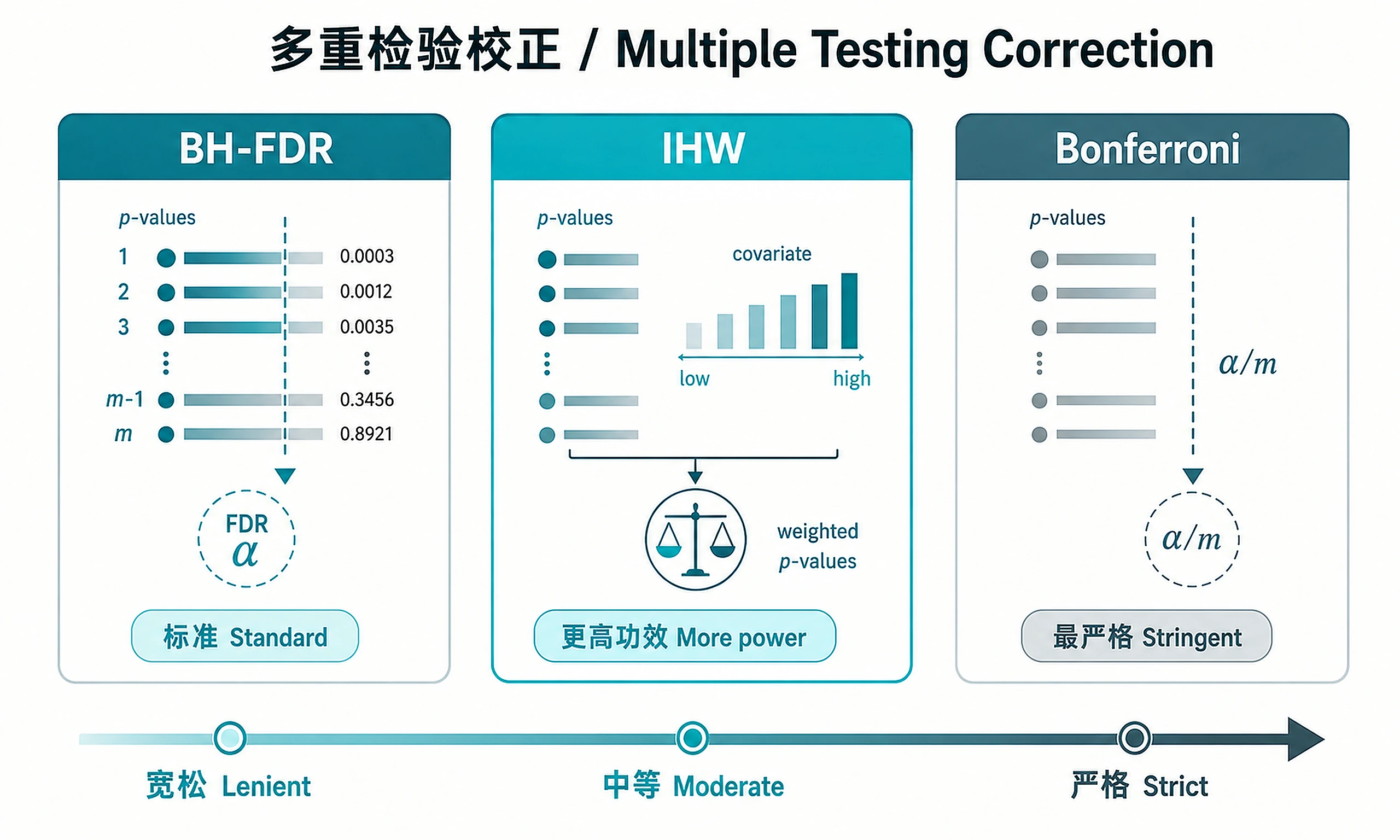
- Multiple testing: BH-FDR (standard), IHW (more power), Bonferroni (stringent), or need guidance
6. Practical Constraints
- Budget: Maximum samples or runs
- Sample availability: Limited? Account for failures (add 10-20% buffer)?
- Batch structure: Processed in batches? Batch size?
- Sequencing depth: Target reads (RNA-seq: 15-30M, ATAC-seq: 25-50M, scRNA-seq: 50-100K/cell)
7. Primary Objective
- Power analysis, sample size determination, batch design, multiple testing guidance, complete design, or budget optimization
Comprehensive clarification guide: references/experimental_design_best_practices.md#clarification-questions
Standard Workflow
🚨 MANDATORY: USE SCRIPTS EXACTLY AS SHOWN - DO NOT WRITE INLINE CODE 🚨
The experimental design workflow follows 4 steps: Load → Calculate → Visualize → Export
Step 1 - Load Parameters
source("scripts/load_example_data.R")
pilot_data <- load_example_data()
With pilot data (preferred):
- Uses
pilot_data$ddsfor power calculations - Uses
pilot_data$cv$medianfor sample size estimation - Provides realistic variability estimates
Without pilot data (alternative):
source("scripts/load_example_data.R")
cv_db <- load_cv_database()
# Select appropriate tissue type from cv_db
✅ VERIFICATION: You MUST see: "✓ Example pilot data loaded successfully!"
Decision: Pilot data provides more accurate estimates. See power_analysis_guidelines.md#pilot-vs-literature
Step 2 - Calculate Design
DO NOT write inline calculation code. Use the provided scripts.
A. Power Analysis - Calculate power for your proposed design
source("scripts/power_rnaseq.R")
power_result <- calc_power_rnaseq(
  depth = 20,
  n_per_group = 6,
  cv = pilot_data$cv$median,
  fold_change = 2,
  alpha = 0.05
)
DO NOT write inline power calculation code. Just source the script and call the function.
B. Sample Size Determination - Calculate required n from pilot data
source("scripts/sample_size_de.R")
required_n <- samplesize_from_pilot(
  pilot_dds = pilot_data$dds,
  fold_change = 1.5,
  power = 0.8,
  fdr = 0.05
)
DO NOT write inline sample size code. Use the function from the script.
C. Batch Assignment - Generate balanced batch layout
source("scripts/batch_assignment.R")
batch_design <- assign_samples_to_batches(
  metadata = pilot_data$metadata,
  batch_size = 8,
  balance_vars = c("condition", "sex")
)
DO NOT manually create batch assignments. Use the OSAT-optimized function.
⚠️ CRITICAL - DO NOT:
- ❌ Write inline power calculation code → STOP: Use calc_power_rnaseq()
- ❌ Write inline plotting code (ggsave, ggplot, etc.) → STOP: Use visualization scripts
- ❌ Manually assign samples to batches → STOP: Use assign_samples_to_batches()
- ❌ Write custom balancing algorithms → STOP: Script uses OSAT's optimal algorithms
- ❌ Try to install svglite → scripts handle SVG fallback automatically
⚠️ IF SCRIPTS FAIL - Script Failure Hierarchy:
- Fix and Retry (90%) - Install missing package, re-run script
- Modify Script (5%) - Edit the script file itself, document changes
- Use as Reference (4%) - Read script, adapt approach, cite source
- Write from Scratch (1%) - Only if genuinely impossible, explain why
NEVER skip directly to writing inline code without trying the script first.
✅ VERIFICATION: You should see:
- After power analysis:
"✓ Power analysis completed successfully!" - After sample size:
"✓ Sample size calculation completed successfully!" - After batch design:
"✓ Batch design generated successfully!"
CRITICAL RULE: Batch must NEVER confound with condition. See batch_effect_mitigation.md#cardinal-rule
Decision points:
- Power ≥0.80? If not, increase n or adjust expectations. See power_analysis_guidelines.md#interpreting-power
- Required n exceed budget? See budget optimization
- Confounding detected? Regenerate with different constraints. See batch_effect_mitigation.md#troubleshooting
Step 3 - Visualize Design
A. Generate power curves:
source("scripts/plot_power_curves.R")
plot_power_vs_samplesize(
  cv = pilot_data$cv$median,
  fold_changes = c(1.5, 2, 3),
  depth = 20,
  output_file = "design_results/power_vs_n"
)
B. Validate and visualize batch design:
source("scripts/batch_validation.R")
confounding_check <- check_confounding(batch_design, "condition")
visualize_batch_design(
  batch_design,
  condition_var = "condition",
  output_file = "design_results/batch_design"
)
DO NOT write inline plotting code (ggsave, ggplot, etc.). Use the visualization scripts.
The scripts handle PNG + SVG export with graceful fallback for SVG dependencies.
✅ VERIFICATION: You should see:
"Saving power curve plots:"followed by PNG + SVG file paths"PASS: No confounding detected"or"WARNING: Batch is CONFOUNDED""Saving batch design plots:"followed by PNG + SVG file paths
Output formats: Always generates both PNG (for presentations) and SVG (for publications) with graceful fallback.
Step 4 - Export All Results
source("scripts/export_design.R")
export_complete_design(batch_design, design_params, output_dir = "design_results")
DO NOT write custom export code. Use export_complete_design().
✅ VERIFICATION: You MUST see: "=== Export Complete ==="
This will generate:
batch_layout_for_lab.csv- Lab-ready sample assignmentsstatistical_analysis_plan.md- Pre-registration analysis planlab_protocol_checklist.md- Lab processing checklistbatch_design.rds- Batch design object (for downstream use)design_parameters.rds- Design parameters (for downstream use)design_parameters.json- Design parameters (human-readable)
RDS objects are CRITICAL for downstream workflows and validation studies.
Complete Workflow Example
For a complete experimental design with all steps:
# Step 1: Load pilot data
source("scripts/load_example_data.R")
pilot_data <- load_example_data()

# Step 2: Calculate design parameters
source("scripts/power_rnaseq.R")
source("scripts/sample_size_de.R")
source("scripts/batch_assignment.R")

power_result <- calc_power_rnaseq(depth = 20, n_per_group = 6, cv = 0.4, fold_change = 2)
required_n <- samplesize_from_pilot(pilot_data$dds, fold_change = 1.5, power = 0.8)
batch_design <- assign_samples_to_batches(pilot_data$metadata, batch_size = 8,
                                          balance_vars = c("condition"))

# Step 3: Visualize and validate
source("scripts/plot_power_curves.R")
source("scripts/batch_validation.R")

plot_power_vs_samplesize(cv = 0.4, fold_changes = c(1.5, 2, 3),
                         output_file = "design_results/power_vs_n")
check_confounding(batch_design, "condition")
visualize_batch_design(batch_design, "condition", output_file = "design_results/batch_design")

# Step 4: Export all results
source("scripts/export_design.R")
design_params <- list(assay = "RNA-seq", conditions = c("control", "treated"),
                     n_per_group = 6, power = 0.85, alpha = 0.05,
                     effect_size = 2, multiple_testing = "BH-FDR")
export_complete_design(batch_design, design_params, output_dir = "design_results")
Note: Specific parameters depend on your experimental requirements (see Clarification Questions).
Decision Guide
Three critical decisions:
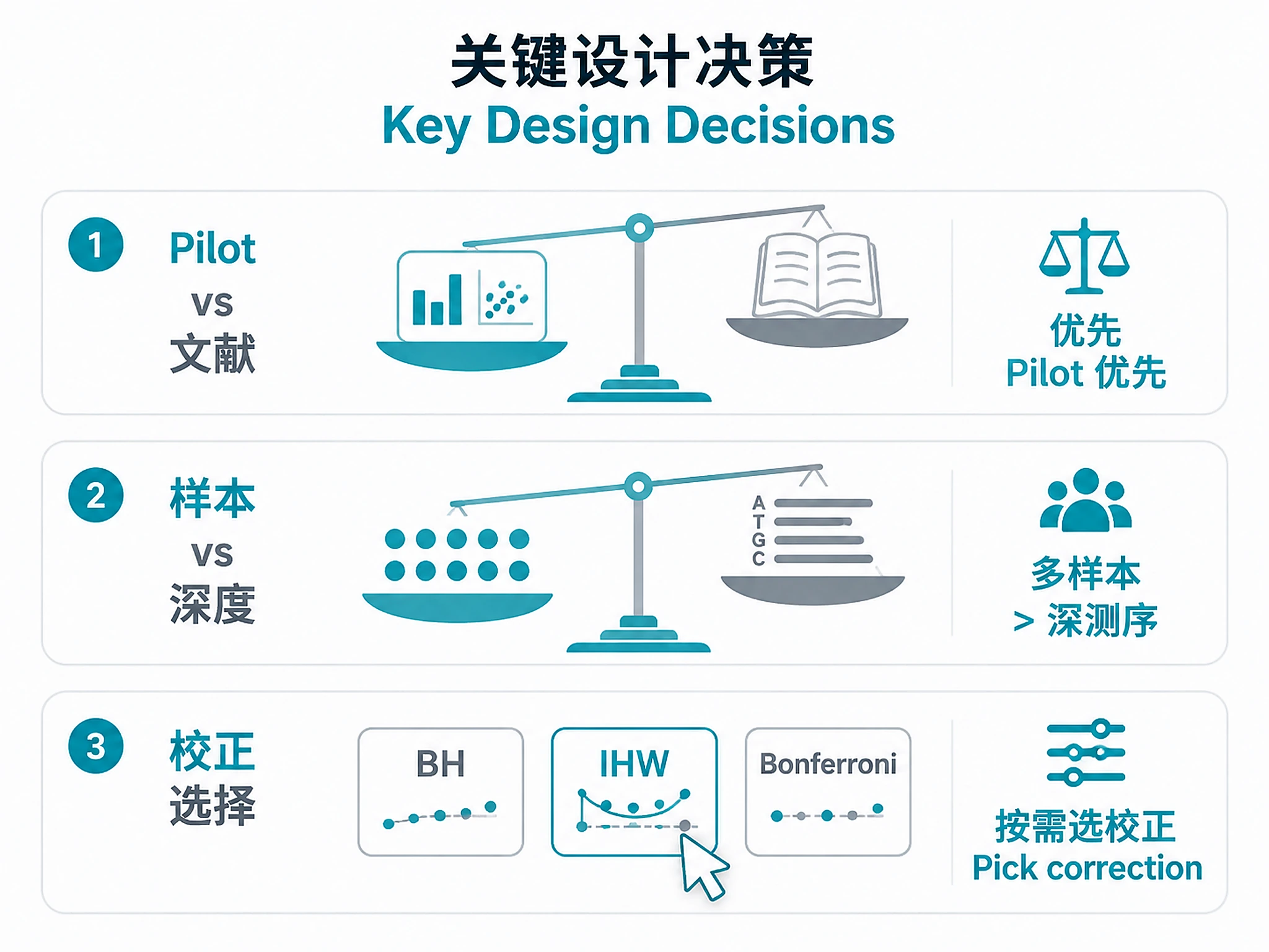
- Pilot vs Literature: Use pilot data if available (more accurate). Literature CV acceptable as fallback.
- Sample Size vs Depth: Prioritize more samples over deeper sequencing for DE. 15-20M reads sufficient for RNA-seq.
- Multiple Testing: BH-FDR (standard), IHW (more power), Bonferroni (stringent).
See: experimental_design_best_practices.md#decision-guide for comprehensive guidance and common usage patterns (power analysis only, batch design only, budget optimization).
Common Issues
| Issue | Cause | Solution |
|---|---|---|
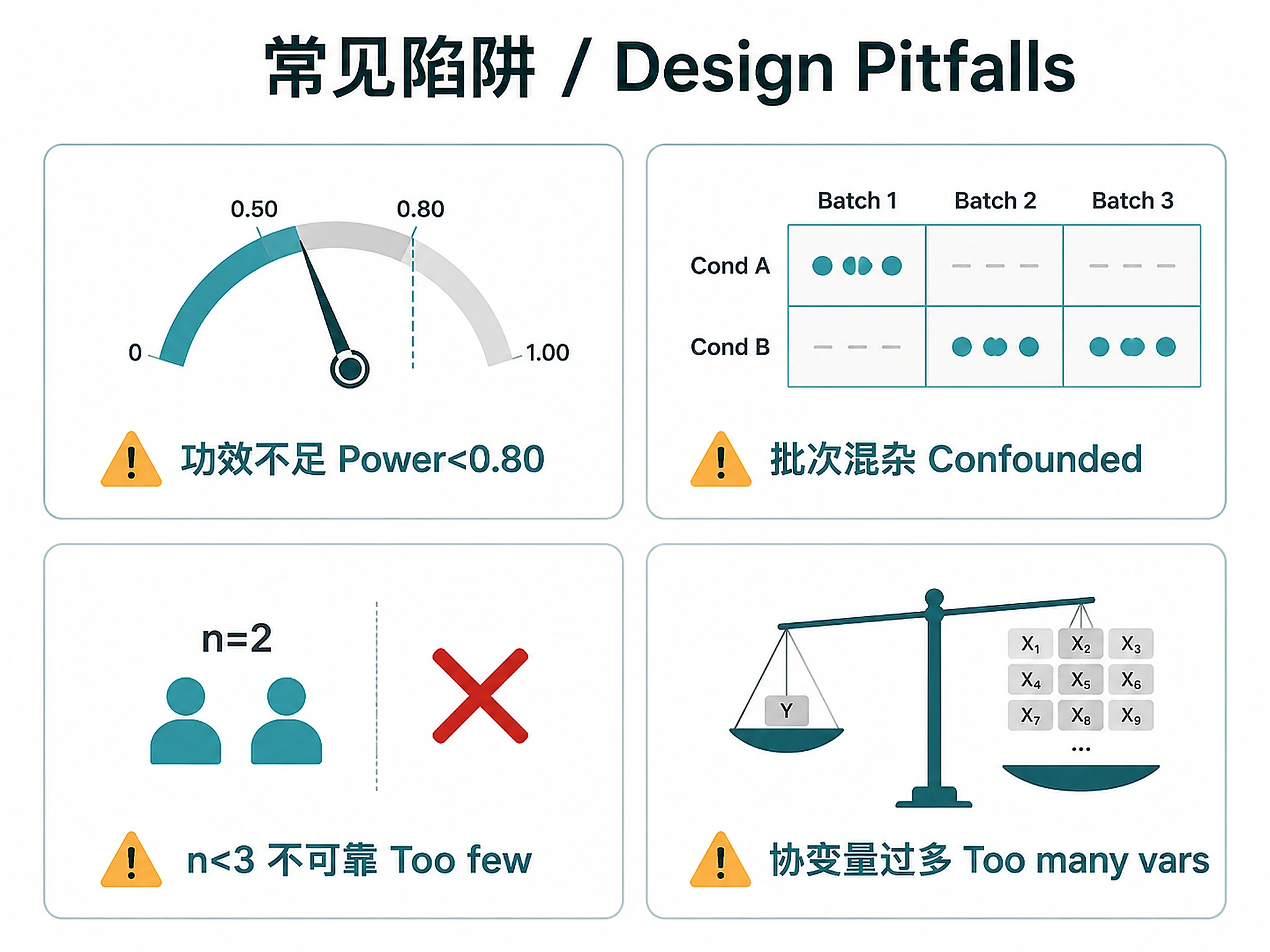
| Power <0.80 with max budget | Effect size too small or CV too high | Increase n, increase depth, or revise effect size expectations. See references/power_analysis_guidelines.md#low-power |
| Batch confounding detected | Unequal condition distribution across batches | Regenerate with stricter balance constraints or adjust batch size. See references/batch_effect_mitigation.md#troubleshooting |
| Required n exceeds sample availability | Pilot data shows high variability or small effect | Consider paired design, blocking by major covariates, or revise target fold-change. See references/experimental_design_best_practices.md#budget-optimization |
| Can't balance all covariates | Too many variables for batch size | Prioritize key covariates (condition > sex > age > others). Some minor imbalance acceptable. See references/batch_effect_mitigation.md#covariate-priority |
| CV estimate varies widely | Pilot data has outliers or low counts | Filter low-count genes (mean <10) before CV calculation. Use median, not mean CV. See references/power_analysis_guidelines.md#cv-estimation |
| Power calculations give n<3 | Very large effect size or low variability | Warning: n<3 too low for valid inference. Plan for minimum n=3-4 even if calculations suggest n=2 |
| Multiple testing correction too stringent | Many tests, low discovery rate | Consider IHW (more powerful than BH-FDR) or independent filtering. See references/multiple_testing_guide.md#choosing |
Detailed troubleshooting: references/troubleshooting_guide.md
Suggested Next Steps
After completing experimental design:
- Execute Experiment - Use batch assignment file to guide sample processing
- Perform DE Analysis - Use bulk-rnaseq-counts-to-de-deseq2, scrnaseq-scanpy-core-analysis, or appropriate skill
- Apply Multiple Testing - Use pre-specified correction method from statistical plan
- Validate Results - Check batch effects were controlled, verify power calculations
Related Skills
Upstream: None - this is typically the first step in a project
Downstream (after data collection):
- bulk-rnaseq-counts-to-de-deseq2 - Differential expression analysis
- functional-enrichment-from-degs - Pathway analysis
- de-results-to-plots - Visualization
Alternative/complementary:
- bulk-omics-clustering - Discover natural groupings post-hoc
- batch-correction-combat - Computational batch correction if needed
References
Detailed documentation:
- references/experimental_design_best_practices.md - General design principles, decision guide, common patterns
- references/power_analysis_guidelines.md - Detailed power calculation methods, pilot vs literature
- references/batch_effect_mitigation.md - Preventing/controlling batch effects, cardinal rule, troubleshooting
- references/multiple_testing_guide.md - Choosing correction methods
- references/qc_guidelines.md - Quality control checkpoints
- references/troubleshooting_guide.md - Common problems and solutions
- references/software_requirements.md - Installation and licenses
- references/cv_tissue_database.csv - Tissue-specific variability estimates
Scripts: See scripts/ directory for all analysis functions:
- Data loading: load_example_data.R
- Power/sample size: power_rnaseq.R, power_atacseq.R, sample_size_de.R, sample_size_scrna.R
- Batch design: batch_assignment.R, batch_validation.R
- Visualization: plot_power_curves.R
- Export: export_design.R (includes RDS saving)
Key Papers:
- Hart SN et al. (2013) J Comput Biol 20(12):970-978 - RNA-seq sample size
- Schurch NJ et al. (2016) RNA 22(6):839-851 - Biological replicates needed
- Leek JT et al. (2010) Nat Rev Genet 11(10):733-739 - Batch effects impact
- Benjamini & Hochberg (1995) J R Stat Soc Series B 57(1):289-300 - FDR control
- Love MI et al. (2014) Genome Biol 15(12):550 - DESeq2 methods
Code preview
scripts/batch_assignment.R
# Batch Assignment Functions
# Create balanced batch designs preventing confounding
# Based on: Leek et al. (2010) Nat Rev Genet and osat package

#' Assign samples to batches with optimal balance
#'
#' @param metadata Data frame with sample metadata (must include sample IDs)
#' @param batch_size Number of samples per batch
#' @param balance_vars Vector of column names to balance across batches
#' @param sample_id_col Name of sample ID column (default: "sample_id")
#' @return Data frame with batch assignments added
#' @export
#' @examples
#' # Create sample metadata
#' metadata <- data.frame(
#'   sample_id = paste0("S", 1:24),
#'   condition = rep(c("Control", "Treatment"), each = 12),
#'   sex = rep(c("M", "F"), 12),
#'   age_group = rep(c("Young", "Old"), each = 12)
#' )
#'
#' # Generate balanced batch assignment
#' batch_design <- assign_samples_to_batches(
#'   metadata = metadata,
#'   batch_size = 8,
#'   balance_vars = c("condition", "sex", "age_group")
#' )
assign_samples_to_batches <- function(metadata,
                                      batch_size,
                                      balance_vars,
                                      sample_id_col = "sample_id") {

  if (!requireNamespace("OSAT", quietly = TRUE)) {
    stop("Package 'OSAT' is required. Install with BiocManager::install('OSAT')")
  }

  # Validate inputs
  if (!sample_id_col %in% colnames(metadata)) {
    stop(paste0("Column '", sample_id_col, "' not found in metadata"))
  }

  missing_vars <- balance_vars[!balance_vars %in% colnames(metadata)]
  if (length(missing_vars) > 0) {
    stop(paste0("Balance variables not found in metadata: ", paste(missing_vars, collapse = ", ")))
  }

  if (batch_size <= 0 || batch_size > nrow(metadata)) {
    stop("Invalid batch_size: must be positive and <= number of samples")
  }

  # Calculate number of batches
  n_batches <- ceiling(nrow(metadata) / batch_size)

  # Prepare data for osat
  sample_ids <- metadata[[sample_id_col]]

  # Create factor variables for balancing
  balance_data <- metadata[, balance_vars, drop = FALSE]

  # Convert all balance variables to factors
  balance_data <- as.data.frame(lapply(balance_data, as.factor))

  # Use osat to generate optimal assignment
  message("Generating optimal batch assignment...")

  tryCatch({
    # Run osat optimization
    osat_result <- OSAT::osat(
      x = balance_data,
      batch.size = batch_size,
      n.batch = n_batches
    )

    # Extract batch assignments
    batch_assignments <- osat_result$BatchLabel

    # Add batch column to metadata
    metadata$batch <- batch_assignments

    # Reorder by batch for convenience
scripts/batch_validation.R
# Batch Design Validation Functions
# Validate batch assignments to prevent confounding and check balance

#' Internal helper to save plots in both PNG and SVG formats
#' @param plot ggplot object
#' @param base_path Base file path (extension will be replaced)
#' @param width Plot width in inches
#' @param height Plot height in inches
#' @param dpi Resolution for PNG
.save_plot <- function(plot, base_path, width = 8, height = 6, dpi = 300) {
  # Always save PNG
  png_path <- sub("\\.(svg|png)$", ".png", base_path)
  ggplot2::ggsave(png_path, plot = plot, width = width, height = height, dpi = dpi, device = "png")
  cat("   Saved:", png_path, "\n")

  # Always try SVG - try ggsave first, fall back to svg() device
  svg_path <- sub("\\.(svg|png)$", ".svg", base_path)
  tryCatch({
    ggplot2::ggsave(svg_path, plot = plot, width = width, height = height, device = "svg")
    cat("   Saved:", svg_path, "\n")
  }, error = function(e) {
    # If ggsave fails, try base R svg() device directly
    tryCatch({
      svg(svg_path, width = width, height = height)
      print(plot)
      dev.off()
      cat("   Saved:", svg_path, "\n")
    }, error = function(e2) {
      cat("   (SVG export failed)\n")
    })
  })
}

#' Check for confounding between batch and condition
#'
#' @param batch_assignment Data frame with batch assignments
#' @param condition_var Name of condition variable column
#' @param batch_var Name of batch variable column (default: "batch")
#' @return List with test results and interpretation
#' @export
#' @examples
#' # Check if batch is confounded with condition
#' # confounding_check <- check_confounding(batch_design, "condition")
check_confounding <- function(batch_assignment,
                              condition_var,
                              batch_var = "batch") {

  # Validate inputs
  if (!condition_var %in% colnames(batch_assignment)) {
    stop(paste0("Condition variable '", condition_var, "' not found in data"))
  }

  if (!batch_var %in% colnames(batch_assignment)) {
    stop(paste0("Batch variable '", batch_var, "' not found in data"))
  }

  # Create contingency table
  cont_table <- table(batch_assignment[[batch_var]], batch_assignment[[condition_var]])

  # Perform chi-square test
  chi_test <- chisq.test(cont_table)

  # Interpretation
  is_confounded <- chi_test$p.value < 0.05

  if (is_confounded) {
    result_message <- paste0(
      "WARNING: Batch is CONFOUNDED with ", condition_var, "!\n",
      "Chi-square test p-value: ", format(chi_test$p.value, digits = 4), " < 0.05\n",
      "This design will not allow separation of batch effects from biological effects.\n",
      "RECOMMENDATION: Regenerate batch assignment."
    )
    status <- "FAILED"
  } else {
    result_message <- paste0(
      "PASS: No confounding detected between batch and ", condition_var, "\n",
      "Chi-square test p-value: ", format(chi_test$p.value, digits = 4), " > 0.05\n",
      "Batch effects can be separated from biological effects."
    )
    status <- "PASSED"
scripts/export_design.R
# Export Experimental Design Functions
# Generate lab-ready files and documentation

#' Export batch assignment layout for lab use
#'
#' @param batch_assignment Data frame with batch assignments
#' @param output_file Output CSV file path
#' @export
export_batch_layout <- function(batch_assignment, output_file = "batch_layout_for_lab.csv") {

  # Reorder columns for lab convenience
  priority_cols <- c("sample_id", "batch", "condition", "processing_order",
                     "plate", "well", "overall_sequence")

  # Get columns that exist
  existing_priority <- priority_cols[priority_cols %in% colnames(batch_assignment)]
  other_cols <- setdiff(colnames(batch_assignment), existing_priority)

  # Reorder
  export_data <- batch_assignment[, c(existing_priority, other_cols)]

  # Sort by batch and processing order (if available)
  if ("batch" %in% colnames(export_data)) {
    if ("processing_order" %in% colnames(export_data)) {
      export_data <- export_data[order(export_data$batch, export_data$processing_order), ]
    } else {
      export_data <- export_data[order(export_data$batch), ]
    }
  }

  # Write CSV
  write.csv(export_data, output_file, row.names = FALSE)

  message(paste0("Batch layout exported to: ", output_file))
  message(paste0("Samples: ", nrow(export_data)))
  message(paste0("Batches: ", length(unique(export_data$batch))))

  # Return invisibly
  invisible(export_data)
}


#' Export statistical analysis plan
#'
#' @param design_params List with experimental design parameters
#' @param output_file Output markdown file path
#' @export
export_statistical_plan <- function(design_params, output_file = "statistical_analysis_plan.md") {

  # Create markdown document
  plan_text <- paste0(
    "# Statistical Analysis Plan\n\n",
    "**Generated:** ", format(Sys.time(), "%Y-%m-%d %H:%M:%S"), "\n\n",
    "---\n\n",
    "## Experimental Design\n\n",
    "**Assay Type:** ", design_params$assay, "\n\n",
    "**Experimental Groups:**\n",
    "- ", paste(design_params$conditions, collapse = "\n- "), "\n\n",
    "**Sample Size:** ", design_params$n_per_group, " biological replicates per group (",
    design_params$n_per_group * length(design_params$conditions), " total samples)\n\n"
  )

  # Add batch information if present
  if (!is.null(design_params$batches)) {
    plan_text <- paste0(
      plan_text,
      "**Batch Structure:** ", design_params$batches, " processing batches\n",
      "- Each batch contains all experimental conditions to prevent confounding\n\n"
    )
  }

  # Add power analysis results
  if (!is.null(design_params$power)) {
    plan_text <- paste0(
      plan_text,
      "## Power Analysis\n\n",
      "**Statistical Power:** ", round(design_params$power, 3), "\n",
      "**Minimum Detectable Effect:** ", design_params$effect_size, "-fold change\n",
      "**Significance Threshold:** α = ", design_params$alpha, "\n\n"
    )
Companion files
| Type | Path | Bytes |
|---|---|---|
| Markdown | references/batch_effect_mitigation.md | 18,688 |
| CSV | references/cv_tissue_database.csv | 2,369 |
| Markdown | references/experimental_design_best_practices.md | 15,613 |
| Markdown | references/multiple_testing_guide.md | 20,952 |
| Markdown | references/power_analysis_guidelines.md | 19,065 |
| Markdown | references/qc_guidelines.md | 8,831 |
| Markdown | references/software_requirements.md | 8,019 |
| Markdown | references/troubleshooting_guide.md | 11,784 |
| R | scripts/batch_assignment.R | 9,753 |
| R | scripts/batch_validation.R | 11,129 |
| R | scripts/export_design.R | 13,384 |
| R | scripts/load_example_data.R | 6,609 |
| R | scripts/multiple_testing.R | 13,095 |
| R | scripts/plot_power_curves.R | 10,867 |
| R | scripts/power_atacseq.R | 6,992 |
| R | scripts/power_pilot_based.R | 9,167 |
| R | scripts/power_rnaseq.R | 7,418 |
| R | scripts/sample_size_de.R | 9,863 |
| R | scripts/sample_size_scrna.R | 10,113 |
| Markdown | SKILL.md | 18,002 |
| JSON | skill.meta.json | 3,885 |