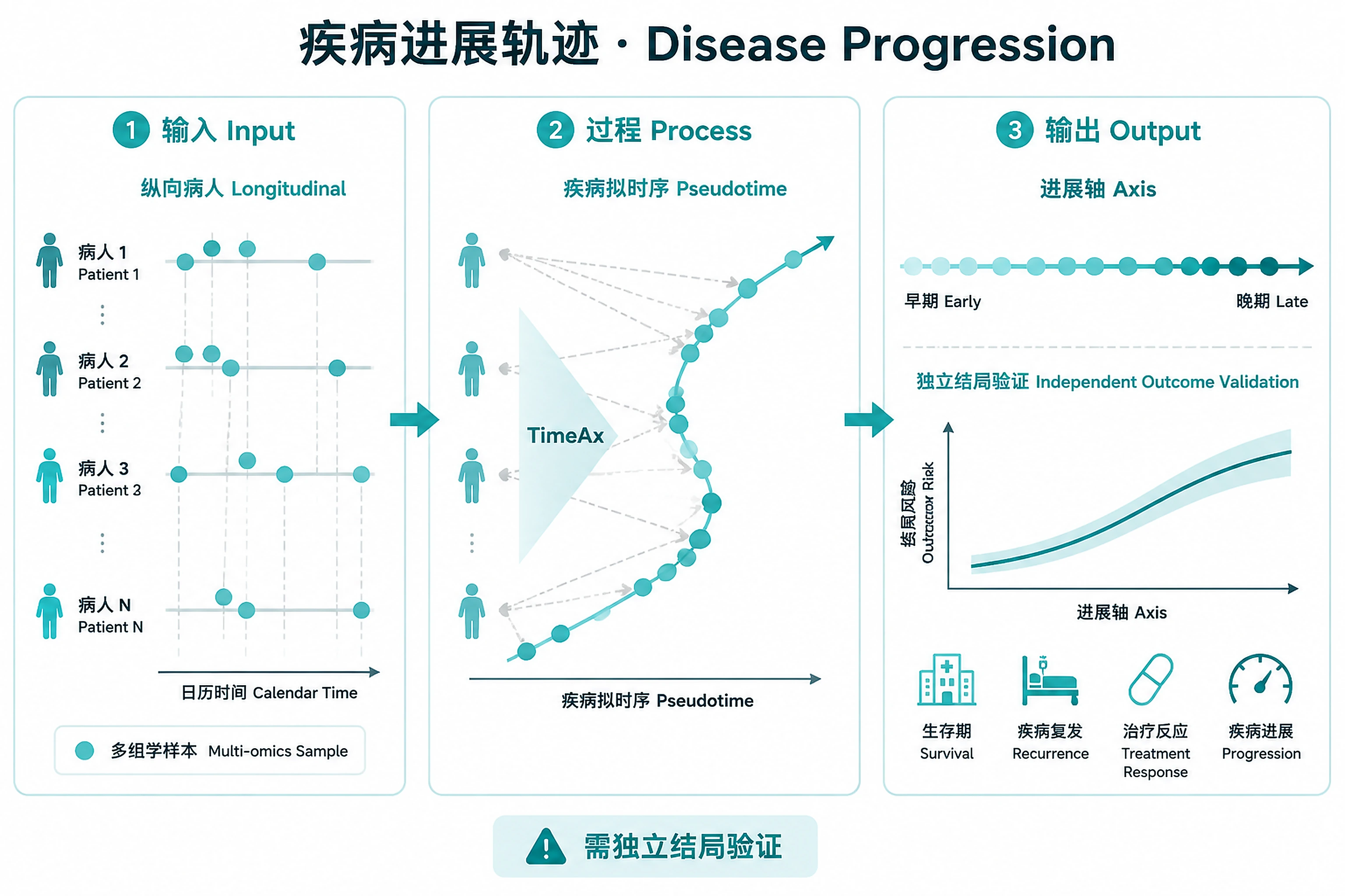
Disease Progression
Reconstruct disease trajectories from longitudinal patient omics.
Overview
Problem. Align irregular patient samples onto one progression axis.
Learning goals
- Like scRNA pseudotime, but for patients
- Validate the axis against independent outcomes
Figures
Tutorial
When to Use This Skill
Use this skill when you have longitudinal patient omics data and want to:
- ✅ Reconstruct disease progression trajectories from time-series data
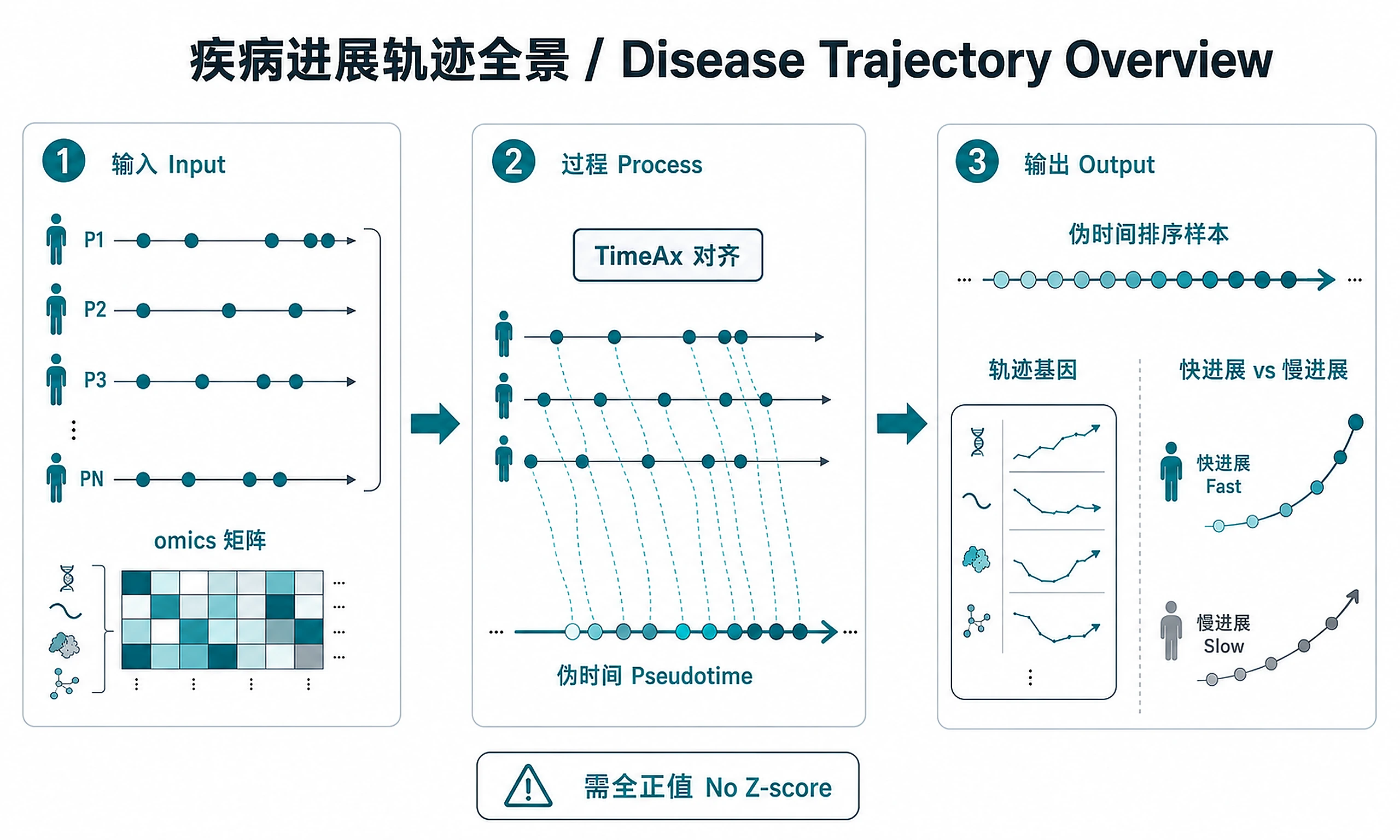
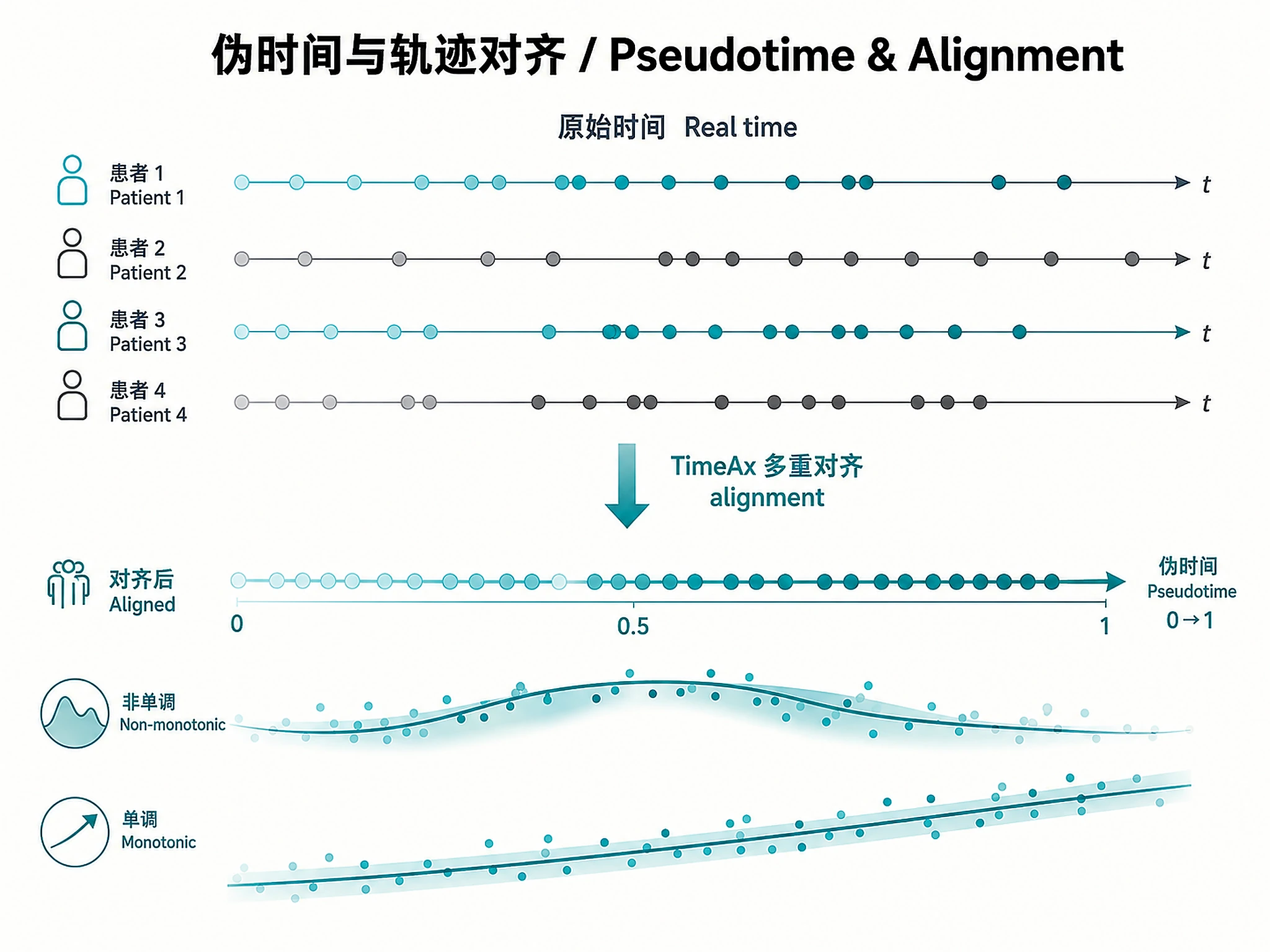
- ✅ Order samples by disease stage (pseudotime) with irregular sampling
- ✅ Identify biomarkers changing along disease trajectory
- ✅ Stratify patients as fast vs. slow progressors
- ✅ Predict clinical outcomes from trajectory position
- ✅ Validate computational staging against clinical measures
Required data:
- Minimum 10 patients with 3+ timepoints each
- Omics data: RNA-seq, proteomics, metabolomics, or clinical biomarkers
- Metadata: Patient IDs, timepoints (days/months/years), optional outcomes
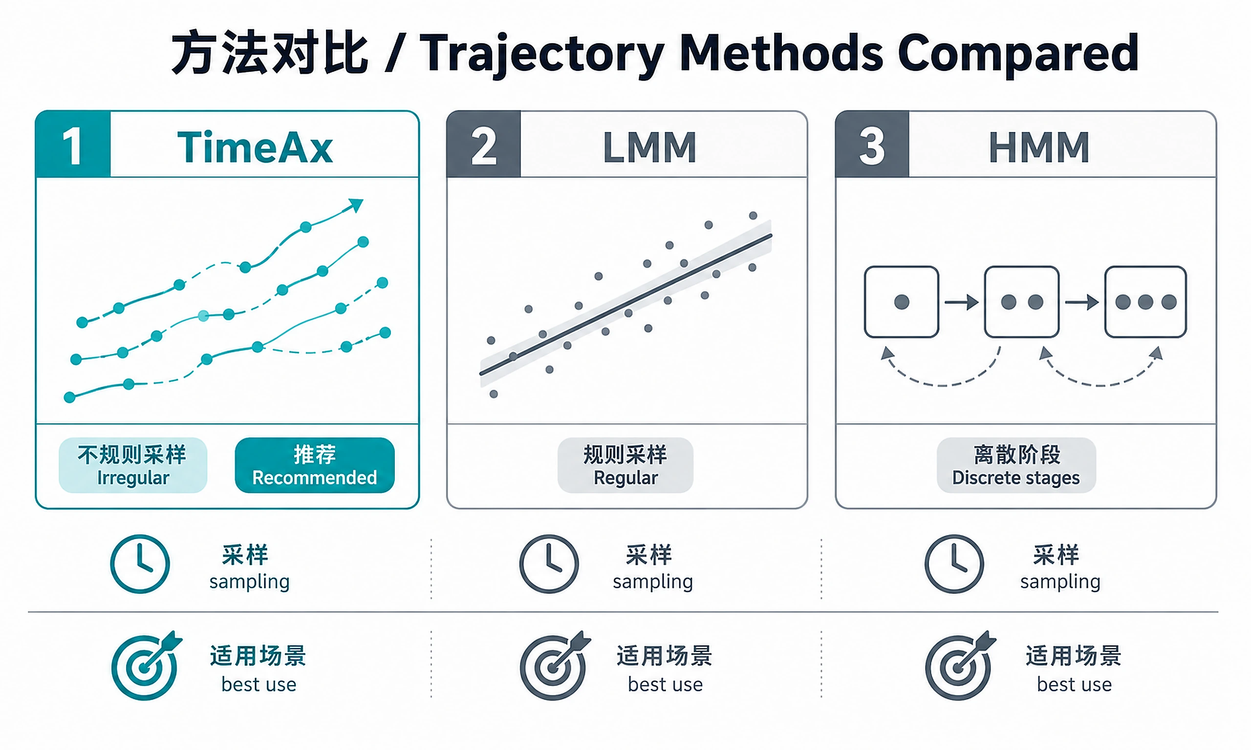
Primary method: TimeAx multiple trajectory alignment (handles irregular sampling)
Feature identification: Polynomial regression (linear/quadratic/cubic) per the TimeAx paper (Frishberg et al., Nat Commun 2023), with FDR-corrected Q-value filtering. Captures both monotonic and non-monotonic dynamics.
Alternative methods: Linear Mixed Models (regular sampling), Hidden Markov Models (discrete stages)
Installation
R ≥ 4.0 with the TimeAx package (primary trajectory method):
# Install TimeAx from GitHub
install.packages("remotes")
remotes::install_github("amitfrish/TimeAx")

# Required for plotting
install.packages(c("ggplot2", "ggprism"))

# Required for demo dataset (GSE128959 batch correction)
BiocManager::install("sva")
Python ≥ 3.9 for the workflow wrapper and analysis pipeline:
# Core analysis packages
pip install numpy pandas scipy scikit-learn statsmodels lifelines

# Visualization packages
pip install seaborn matplotlib

# PDF report generation (optional)
pip install reportlab

# Optional
pip install hmmlearn        # Hidden Markov Models alternative
For Linear Mixed Models alternative: R packages lme4, lmerTest
License compliance: All packages use permissive licenses (MIT, BSD, Apache 2.0) - commercial AI agent use permitted.
For detailed installation and troubleshooting, see troubleshooting_guide.md
Inputs
Required files:
-
Data matrix (features × samples)
- CSV/TSV format with features as rows, samples as columns
- Feature types: genes, proteins, metabolites, or clinical biomarkers
- Normalized counts or continuous measurements
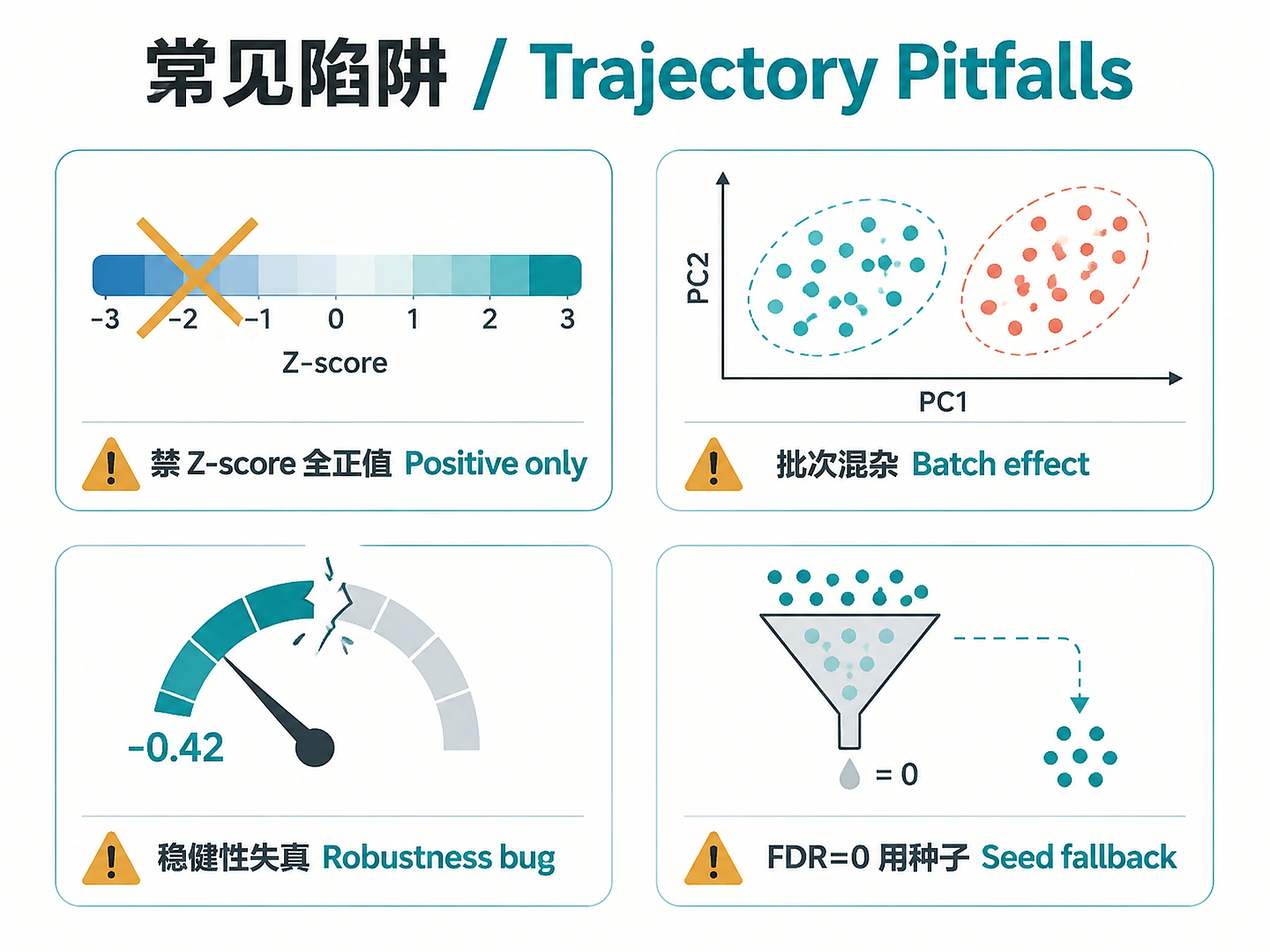
- ⚠️ TimeAx requires all-positive values (e.g., log2-normalized, RMA). Do NOT Z-score normalize before TimeAx — it creates negative values that disable the
ratiomechanism.
-
Sample metadata (CSV/TSV)
- Required columns:
sample_id,patient_id,timepoint - Optional:
outcome,treatment,batch, clinical covariates - Timepoints: numeric values (days, months, years from baseline)
- Required columns:
Data requirements:
- ≥10 patients minimum (20+ recommended)
- ≥3 timepoints per patient minimum
- Handles irregular sampling (different timepoints per patient)
- Works with cross-sectional + longitudinal cohorts
Outputs
Primary results:
pseudotime_assignments.csv- Disease pseudotime for each sampletrajectory_features.csv- Features changing along trajectory, with polynomial degree, R², and directionpatient_summaries.csv- Per-patient progression statisticsall_feature_statistics.csv- Statistics for all tested features
Analysis objects (for downstream use):
timeax_model.pkl- Complete TimeAx model object- Load with:
model = pickle.load(open('timeax_model.pkl', 'rb')) - Required for: Projecting new samples, downstream trajectory analysis
Reports:
analysis_report.pdf- Publication-quality PDF with Introduction, Methods, Results, Conclusions- Requires:
pip install reportlab(optional — markdown report generated regardless) SUMMARY.txt- Plain-text summary report
TimeAx R plots (PNG + SVG, generated in Step 2):
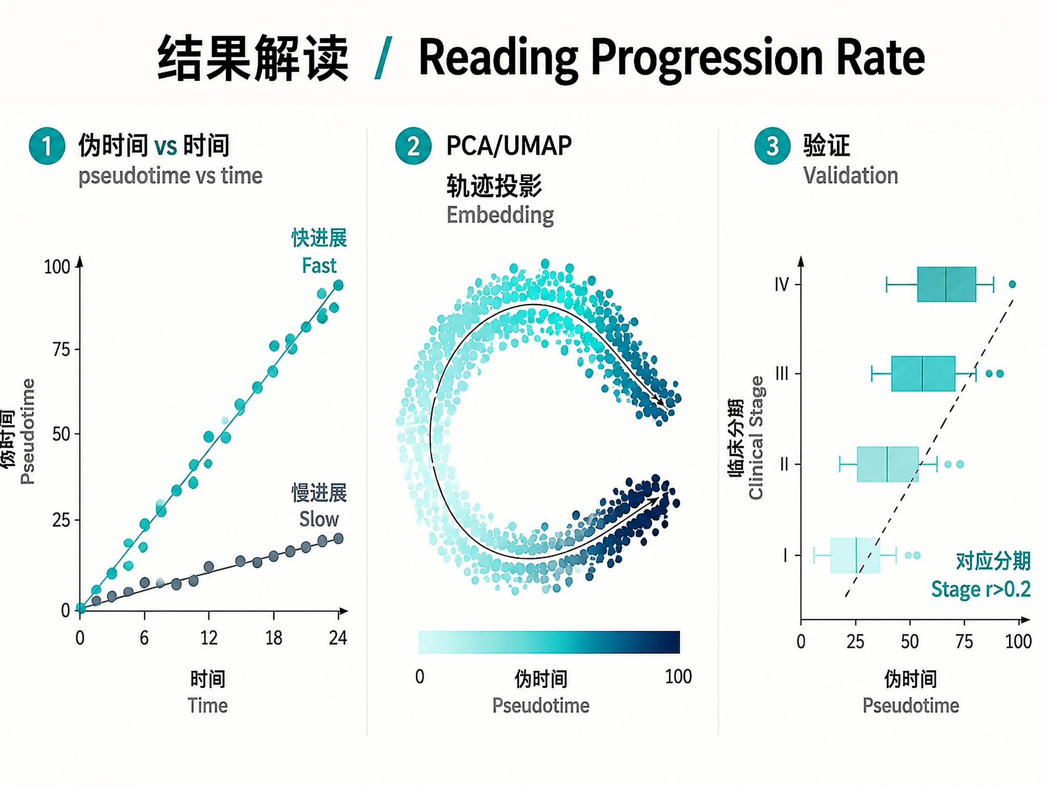
timeax_pseudotime_vs_time.png/.svg- Per-patient pseudotime vs actual time trajectoriestimeax_progression_rates.png/.svg- Patient progression rate comparison (fast vs slow)timeax_seed_dynamics.png/.svg- Seed feature expression trends along pseudotimetimeax_uncertainty.png/.svg- Pseudotime uncertainty distribution
Python plots (PNG + SVG, generated in Step 3):
patient_trajectories_pca.png/.svg- PCA with pseudotime coloring and patient trajectory linespatient_trajectories_umap.png/.svg- UMAP nonlinear projectiontrajectory_heatmap.png/.svg- Feature expression clustermaptrajectory_trends.png/.svg- Polynomial fit trends for top featurespseudotime_vs_stage.png/.svg- Pseudotime vs clinical tumor stage (biological validation)patient_progression.png/.svg- Per-patient pseudotime spaghetti plotseed_feature_heatmap.png/.svg- TimeAx seed feature dynamics heatmap
Metadata:
model_metadata.json- Analysis parameters, quality metrics (monotonicity, robustness)
Clarification Questions
🚨 ALWAYS ask Question 1 FIRST. Do not ask about data type, study design, or analysis parameters before the user has answered Question 1.
1. Input Files (ASK THIS FIRST)
- Do you have longitudinal patient omics data to analyze?
- If uploaded: Are these your data matrix and sample metadata files?
- Expected: Data matrix (features × samples) + metadata (sample_id, patient_id, timepoint)
- Or use example/demo data?
- GSE128959 bladder cancer recurrence (18 patients, 84 samples, 17K genes) — from the TimeAx paper (Frishberg et al. 2023). Requires R +
svapackage. Downloads ~5MB on first run.
- GSE128959 bladder cancer recurrence (18 patients, 84 samples, 17K genes) — from the TimeAx paper (Frishberg et al. 2023). Requires R +
🚨 IF EXAMPLE DATA SELECTED: All parameters are pre-defined (bladder cancer microarray, 18 patients, 4-6 timepoints, tumor recurrence, TimeAx method with ComBat batch correction). DO NOT ask questions 2-6. Proceed directly to Step 1.
Questions 2-6 are ONLY for users providing their own data:
2. Data Type: Bulk RNA-seq, proteomics, metabolomics, clinical biomarkers, or multi-omics?
3. Study Design: Number of patients (min 10, recommend 20+)? Timepoints per patient (min 3)? Sampling pattern (regular/irregular)? Time units and range?
4. Disease Context: Disease type? Treatment status? Available clinical outcomes (survival, relapse, response)? Known clinical staging?
5. Analysis Goals: Pseudotime ordering, patient stratification, biomarker discovery, outcome prediction, or trajectory comparison?
6. Method Preference: TimeAx (recommended), Linear Mixed Models, Hidden Markov Models, or not sure?
Standard Workflow
🚨 MANDATORY: USE SCRIPTS EXACTLY AS SHOWN - DO NOT WRITE INLINE CODE 🚨
Step 1 - Load and preprocess data:
For example/demo data (GSE128959 bladder cancer):
from scripts.load_and_preprocess import load_example_data, load_and_preprocess_data

# Load GSE128959 (downloads and preprocesses via R on first run)
data, metadata = load_example_data()

# Save to files for the standard pipeline
data.to_csv('gse128959_expression.csv')
metadata.to_csv('gse128959_metadata.csv', index=False)

# Run through standard preprocessing
data, metadata, preprocessing_stats = load_and_preprocess_data(
    data_file='gse128959_expression.csv',
    metadata_file='gse128959_metadata.csv',
    data_type='rnaseq',
    min_patients=10,
    min_timepoints=3
)
For your own data:
from scripts.load_and_preprocess import load_and_preprocess_data

data, metadata, preprocessing_stats = load_and_preprocess_data(
    data_file="patient_expression.csv",
    metadata_file="sample_metadata.csv",
    data_type='rnaseq',  # 'rnaseq', 'proteomics', 'metabolomics', 'clinical'
    min_patients=10,
    min_timepoints=3
)
DO NOT write inline data loading or preprocessing code. Just use the script.
✅ VERIFICATION: You MUST see: "✓ Data loaded and preprocessed successfully!"
Step 2 - Run trajectory analysis:
from scripts.run_trajectory_analysis import run_trajectory_analysis

# Run TimeAx alignment and identify trajectory features
results = run_trajectory_analysis(
    data,
    metadata,
    method='timeax',  # 'timeax', 'lmm', 'hmm'
    patient_column='patient_id',
    time_column='timepoint'
)
# Extract: pseudotime, trajectory_features, model, robustness_score
DO NOT write inline TimeAx or trajectory code. Just use the script.
✅ VERIFICATION: You MUST see: "✓ Trajectory analysis completed successfully!"
Step 3 - Generate visualizations:
from scripts.generate_all_plots import generate_all_plots

# Generate all plots (PNG + SVG with graceful fallback)
generate_all_plots(
    data,
    metadata,
    results,
    output_dir='trajectory_results'
)
DO NOT write inline plotting code (plt.savefig, seaborn, etc.). Just use the script.
The script handles PNG + SVG export with graceful fallback for SVG dependencies.
✅ VERIFICATION: You MUST see: "✓ All visualizations generated successfully!"
Step 4 - Export results:
from scripts.export_results import export_all

# Export all results, model object, and metadata
export_all(
    data=data,
    metadata=metadata,
    results=results,
    output_dir='trajectory_results'
)
DO NOT write custom export code. Use export_all().
✅ VERIFICATION: You MUST see: "=== Export Complete ==="
⚠️ CRITICAL - DO NOT:
- ❌ Write inline data loading code → STOP: Use
load_and_preprocess_data() - ❌ Write inline TimeAx/trajectory code → STOP: Use
run_trajectory_analysis() - ❌ Write inline plotting code → STOP: Use
generate_all_plots() - ❌ Write custom export code → STOP: Use
export_all()
⚠️ IF SCRIPTS FAIL - Script Failure Hierarchy:
- Fix and Retry (90%) - Install missing package, re-run script
- Modify Script (5%) - Edit the script file itself, document changes
- Use as Reference (4%) - Read script, adapt approach, cite source
- Write from Scratch (1%) - Only if genuinely impossible, explain why
NEVER skip directly to writing inline code without trying the script first.
Detailed Methodology
For comprehensive details on algorithms, parameters, and methods:
- TimeAx algorithm: timeax_methodology.md
- Alternative methods (LMM, HMM): lmm_hmm_alternatives.md
- Method comparison and selection: method_comparison.md
- Data preprocessing by type: data_preprocessing_guide.md
- Validation framework: validation_framework.md
Quality Control
Quick checklist:
- ✅ ≥10 patients with ≥3 timepoints each
- ✅ Within-patient monotonicity >0.5 (good) or 0.3-0.5 (moderate)
- ✅ Pseudotime correlates with clinical measures (r >0.2, p <0.05)
- ✅ Trajectory features identified (seed feature fallback if FDR <0.05 yields 0)
- ✅ Samples don't cluster by batch (check PCA)
Note on robustness: The TimeAx robustness() function (v0.1.1) can produce misleading negative values even on valid data. Use within-patient monotonicity as the primary quality metric instead.
For comprehensive QC guidelines, see validation_framework.md
Common Issues
| Error | Cause | Solution |
|---|---|---|
| Negative robustness score | Known TimeAx v0.1.1 bug | Normal. The robustness() function is unreliable. Use within-patient monotonicity (>0.5 = good) as the primary quality metric instead. |
| 0 trajectory features (FDR <0.05) | FDR too stringent for genome-wide test | Normal with real data. The script automatically falls back to testing TimeAx seed features (reduced FDR burden) and nominal p < 0.05. |
| Memory error during alignment | Too many features (>20,000) | Reduce to 5000-10000 most variable features before TimeAx. Script does this automatically. |
| SVG export failed | Missing cairo system library | Normal - PNG still generated. Script handles fallback automatically. DO NOT try to install cairo manually. |
| Samples cluster by batch not time | Uncorrected batch effects | Run ComBat batch correction before trajectory analysis. Set batch_correction=True in preprocessing. |
Negative values disable ratio mode |
Z-score or log-fold-change normalization | TimeAx ratio=TRUE requires positive values. Use log2 counts, RMA, or TPM — NOT Z-scores. |
| "R TimeAx not available" | R or TimeAx R package not installed | STOP: Install R, then run: Rscript -e 'remotes::install_github("amitfrish/TimeAx")'. See Installation section. |
| PDF report not generated | reportlab not installed | Normal. Install with pip install reportlab. SUMMARY.txt is always generated as fallback. |
For complete troubleshooting, see troubleshooting_guide.md
Suggested Next Steps
After trajectory analysis, consider these downstream analyses:
-
Functional enrichment → Use
functional-enrichment-gprofilerskill- Input:
trajectory_features.csv(top up/down-regulated features) - Find pathways changing along disease trajectory
- Input:
-
Tissue expression analysis → Use
tissue-expression-from-degsskill- Input:
trajectory_features.csv - Identify tissue-specific trajectory markers
- Input:
-
Transcription factor activity → Use
tf-activity-dorotheaskill- Input:
pseudotime_assignments.csv+ original expression data - Find TFs driving disease progression
- Input:
-
Survival analysis → Built into clinical validation
- Input:
pseudotime_assignments.csv+ survival data - Stratify patients by pseudotime tertiles/quartiles
- Input:
-
Project new samples → Use
scripts/timeax_inference.py- Load:
timeax_model.pkl - Stage new patients on trained trajectory
- Load:
Related Skills
Upstream (data generation):
bulk-rnaseq-counts-to-de-deseq2- Generate expression dataproteomics-differential-expression- Proteomics quantificationmetabolomics-preprocessing- Metabolite data
Downstream (interpretation):
functional-enrichment-gprofiler- Pathway analysis of trajectory featurestissue-expression-from-degs- Tissue-specific markerstf-activity-dorothea- Transcription factor driversgrn-pyscenic- Gene regulatory networks along trajectory
Alternative trajectory methods:
pseudotime-monocle- For single-cell RNA-seq trajectoriestrajectory-inference-slingshot- Branching trajectories
References
Primary Citations
-
TimeAx: Frishberg A, van den Munckhof ICL, Ter Horst R, et al. Reconstructing disease dynamics for mechanistic insights and clinical benefit. Nat Commun. 2023;14(1):6940. https://doi.org/10.1038/s41467-023-42354-8
-
Linear Mixed Models: Bates D, Mächler M, Bolker B, Walker S. Fitting Linear Mixed-Effects Models Using lme4. J Stat Softw. 2015;67(1):1-48.
-
Disease Trajectories Review: Schmidt AF, Heerspink HJL, Denig P, et al. Disease trajectory browser for exploring temporal, population-wide disease progression patterns. Nat Commun. 2020;11:4952.
Software
| Software | Version | License | Commercial Use |
|---|---|---|---|
| TimeAx | ≥0.1.0 | MIT | ✅ Permitted |
| NumPy | ≥1.21 | BSD | ✅ Permitted |
| Pandas | ≥1.3 | BSD | ✅ Permitted |
| scikit-learn | ≥1.0 | BSD | ✅ Permitted |
| seaborn | ≥0.11 | BSD | ✅ Permitted |
| matplotlib | ≥3.5 | BSD | ✅ Permitted |
| ggprism (R) | ≥1.0.3 | GPL (≥3) | ✅ Permitted |
| sva (R) | ≥3.40 | Artistic-2.0 | ✅ Permitted |
| reportlab | ≥3.6 | BSD | ✅ Permitted |
Online Resources
- TimeAx GitHub: https://github.com/amitfrish/TimeAx
- TimeAx Documentation: https://timeax.readthedocs.io/
- Disease Progression Modeling Review: https://www.annualreviews.org/content/journals/10.1146/annurev-biodatasci-110123-041001
Code preview
scripts/clinical_validation.py
"""
Clinical Validation Functions for Disease Progression Trajectories

This module provides functions for validating disease progression trajectories
against clinical measures, outcomes, and staging systems.
"""

import numpy as np
import pandas as pd
from scipy.stats import spearmanr, mannwhitneyu, kruskal
from lifelines import CoxPHFitter, KaplanMeierFitter
from lifelines.statistics import logrank_test
from plotnine import (ggplot, aes, geom_boxplot, geom_step, labs,
                      theme_minimal, facet_wrap)
from plotnine_prism import theme_prism


def correlate_with_clinical_scores(metadata, pseudotime_column='pseudotime',
                                    clinical_columns=None):
    """
    Correlate pseudotime with clinical severity scores.

    Parameters
    ----------
    metadata : pd.DataFrame
        Sample metadata with pseudotime and clinical scores
    pseudotime_column : str
        Column name for pseudotime values
    clinical_columns : list of str, optional
        Clinical score columns to correlate. If None, auto-detect numeric columns.

    Returns
    -------
    pd.DataFrame
        Correlation results with columns: variable, correlation, pvalue
    """
    if clinical_columns is None:
        # Auto-detect numeric columns (excluding pseudotime)
        clinical_columns = metadata.select_dtypes(include=[np.number]).columns
        clinical_columns = [c for c in clinical_columns
                            if c != pseudotime_column and c != 'patient_id']

    results = []

    for col in clinical_columns:
        # Remove missing values
        valid_mask = ~metadata[col].isnull() & ~metadata[pseudotime_column].isnull()
        if valid_mask.sum() < 3:
            continue  # Skip if too few valid pairs

        corr, pval = spearmanr(metadata.loc[valid_mask, pseudotime_column],
                               metadata.loc[valid_mask, col])

        results.append({
            'variable': col,
            'correlation': corr,
            'pvalue': pval,
            'n_samples': valid_mask.sum()
        })

    results_df = pd.DataFrame(results)
    results_df = results_df.sort_values('pvalue')

    # Print summary
    print("Pseudotime vs. Clinical Scores Correlation")
    print("=" * 60)
    for _, row in results_df.iterrows():
        print(f"{row['variable']:30s} r={row['correlation']:6.3f}  p={row['pvalue']:.3e}  n={row['n_samples']}")

    return results_df


def compare_by_clinical_stage(metadata, pseudotime_column='pseudotime',
                               stage_column='clinical_stage',
                               output_file=None):
    """
    Compare pseudotime across discrete clinical stages.

    Parameters
    ----------
scripts/export_results.py
"""
Export all trajectory analysis results and model objects.

This module provides the export_all() function for Step 4 of the standard workflow.
"""

import pandas as pd
import numpy as np
import pickle
import json
import os
from typing import Dict, Optional, List
from datetime import datetime


def export_all(
    data: pd.DataFrame,
    metadata: pd.DataFrame,
    results: Dict,
    output_dir: str = 'trajectory_results',
    include_plots: bool = True
) -> None:
    """
    Export all trajectory analysis results, model objects, and metadata.

    This is the Step 4 function that exports:
    - Pseudotime assignments (CSV)
    - Trajectory features (CSV)
    - Patient summaries (CSV)
    - Model object (pickle) - CRITICAL for downstream use
    - Analysis metadata (JSON)
    - Optional: plots if generated

    Parameters
    ----------
    data : pd.DataFrame
        Preprocessed data matrix (features × samples)
    metadata : pd.DataFrame
        Sample metadata with pseudotime
    results : dict
        Results from run_trajectory_analysis() containing:
        - 'pseudotime': sample pseudotimes
        - 'trajectory_features': significant features
        - 'model': fitted model object
        - 'robustness_score': quality metric
        - 'method': method used
        - 'feature_stats': statistics for all features
    output_dir : str, default='trajectory_results'
        Output directory for all files
    include_plots : bool, default=True
        Whether to copy plot files to export directory

    Returns
    -------
    None
        Saves all outputs to output_dir
    """

    print("\n=== Step 4: Export Results ===\n")

    # Create output directory
    os.makedirs(output_dir, exist_ok=True)

    # Extract results
    pseudotime = results['pseudotime']
    trajectory_features = results['trajectory_features']
    feature_stats = results['feature_stats']
    model = results.get('model')
    robustness_score = results.get('robustness_score')
    monotonicity_score = results.get('monotonicity_score')
    method = results.get('method', 'unknown')

    # 1. Export pseudotime assignments
    print("Exporting pseudotime assignments...")
    pseudotime_df = pd.DataFrame({
        'sample_id': pseudotime.index,
        'pseudotime': pseudotime.values
    })

    # Add metadata columns if available
scripts/generate_all_plots.py
"""
Generate all trajectory visualizations with PNG + SVG export.

This module creates publication-quality plots with graceful SVG fallback.
"""

import pandas as pd
import numpy as np
import matplotlib.pyplot as plt
import seaborn as sns
from typing import Dict, Optional, List
import os
from sklearn.decomposition import PCA

# Set seaborn theme and Helvetica font (project standard)
sns.set_style("ticks")
plt.rcParams['font.family'] = 'sans-serif'
plt.rcParams['font.sans-serif'] = ['Helvetica']

# Try to import UMAP
try:
    from umap import UMAP
    UMAP_AVAILABLE = True
except ImportError:
    UMAP_AVAILABLE = False


def generate_all_plots(
    data: pd.DataFrame,
    metadata: pd.DataFrame,
    results: Dict,
    output_dir: str = 'trajectory_results'
) -> None:
    """
    Generate all trajectory visualizations (PNG + SVG).

    This is the consolidated Step 3 function that creates:
    - PCA trajectory plot
    - UMAP trajectory plot (if available)
    - Trajectory feature heatmap
    - Feature trend plots

    Parameters
    ----------
    data : pd.DataFrame
        Preprocessed data matrix (features × samples)
    metadata : pd.DataFrame
        Sample metadata
    results : dict
        Results from run_trajectory_analysis() containing:
        - 'pseudotime': sample pseudotimes
        - 'trajectory_features': significant features
        - 'robustness_score': quality metric
    output_dir : str, default='trajectory_results'
        Output directory for plots

    Returns
    -------
    None
        Saves plots to output_dir
    """

    print("\n=== Step 3: Generate Visualizations ===\n")

    # Create output directory
    os.makedirs(output_dir, exist_ok=True)

    # Extract results
    pseudotime = results['pseudotime']
    trajectory_features = results['trajectory_features']

    # Add pseudotime to metadata for plotting
    plot_metadata = metadata.copy()
    plot_metadata['pseudotime'] = pseudotime.values

    # 1. PCA trajectory plot (with patient lines)
    print("Generating PCA trajectory plot...")
    try:
        _plot_pca_trajectory(
            data, plot_metadata,
Companion files
| Type | Path | Bytes |
|---|---|---|
| Markdown | references/data_preprocessing_guide.md | 9,949 |
| Markdown | references/lmm_hmm_alternatives.md | 19,544 |
| Markdown | references/method_comparison.md | 11,854 |
| Markdown | references/timeax_methodology.md | 9,954 |
| Markdown | references/troubleshooting_guide.md | 7,456 |
| Markdown | references/validation_framework.md | 18,179 |
| Markdown | references/workflow_integration.md | 18,785 |
| Python | scripts/clinical_validation.py | 17,271 |
| Python | scripts/export_results.py | 15,114 |
| Python | scripts/generate_all_plots.py | 22,187 |
| Python | scripts/generate_report.py | 19,402 |
| Python | scripts/load_and_preprocess.py | 11,643 |
| R | scripts/load_gse128959.R | 4,464 |
| Python | scripts/load_longitudinal_data.py | 8,784 |
| Python | scripts/mock_timeax.py | 7,261 |
| Python | scripts/plot_patient_trajectories.py | 6,915 |
| Python | scripts/preprocess_features.py | 8,822 |
| R | scripts/run_timeax.R | 11,197 |
| Python | scripts/run_trajectory_analysis.py | 18,202 |
| Python | scripts/timeax_alignment.py | 6,508 |
| Python | scripts/timeax_r_wrapper.py | 8,763 |
| Markdown | SKILL.md | 15,821 |
| JSON | skill.meta.json | 4,172 |