Functional Enrichment
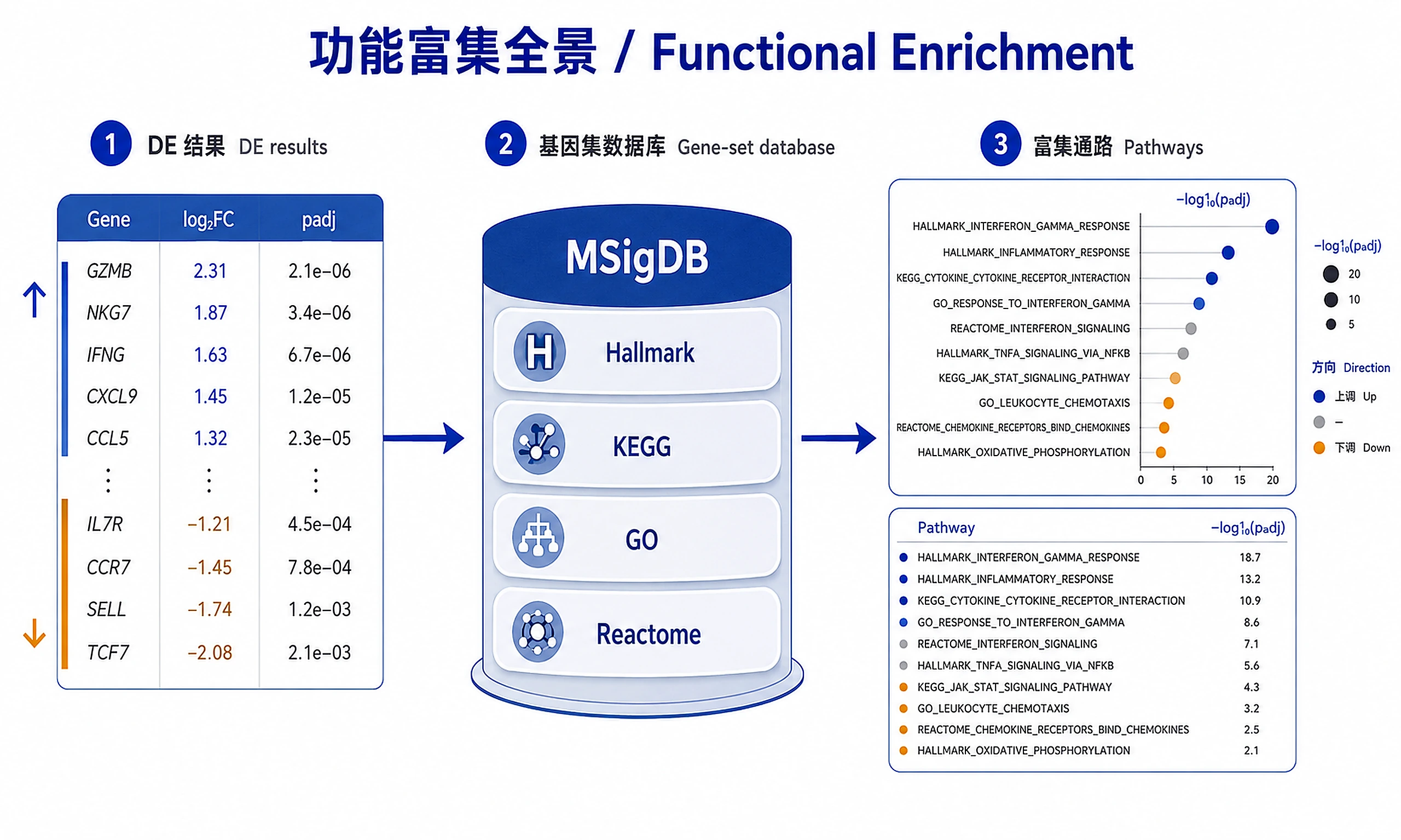
Turn a DE gene list into pathways and GO terms with clusterProfiler.
Overview
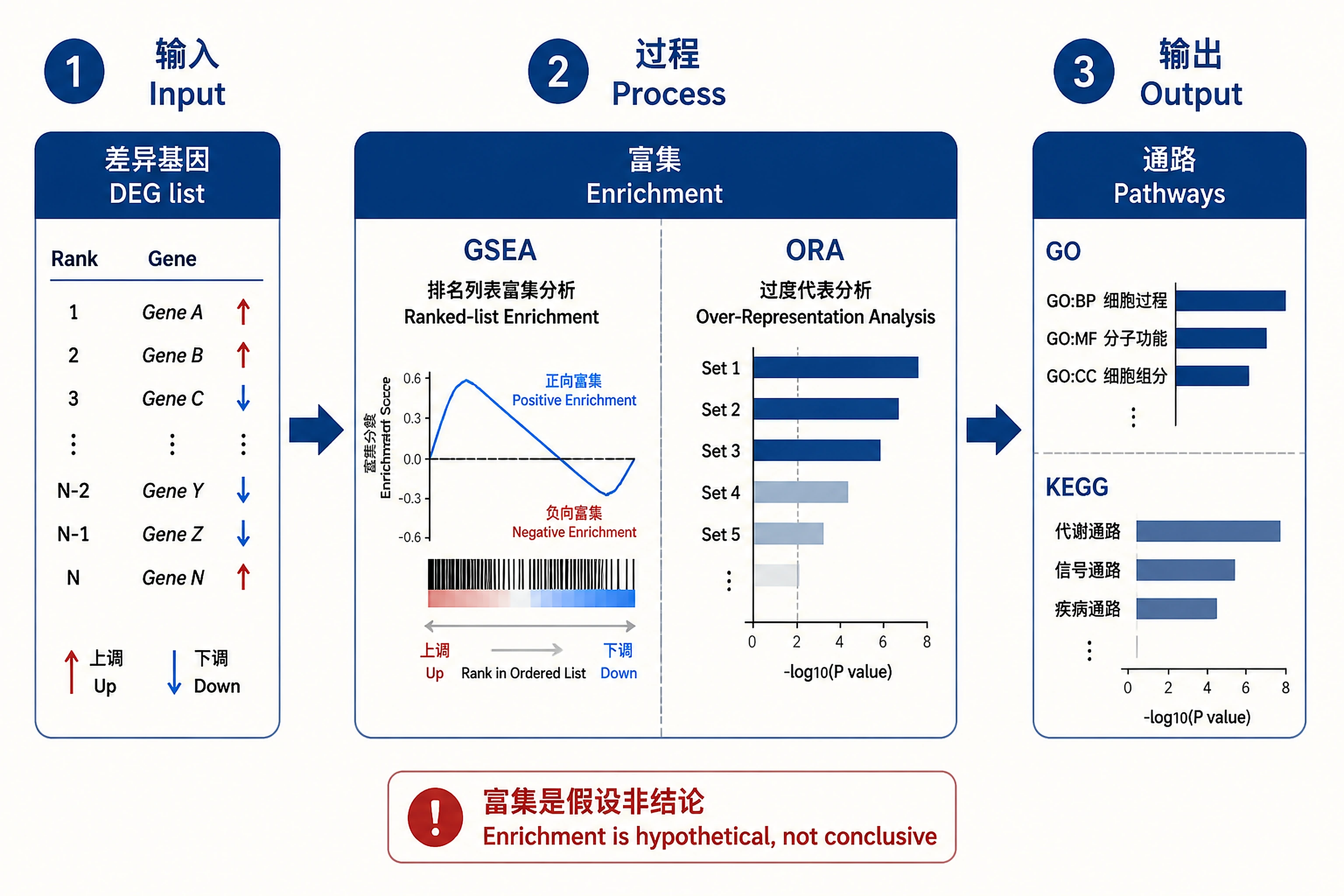
Problem. Translate a long DE list into interpretable pathways.
Learning goals
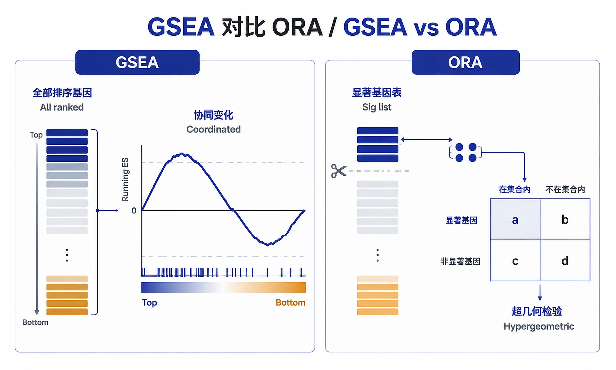
- GSEA (full ranking) vs ORA (thresholded)
- Enrichment generates hypotheses, not conclusions
Figures
Tutorial
Translate differential expression results into biological insights using GSEA and ORA.
When to Use This Skill
Use this skill after completing differential expression analysis to identify enriched pathways and biological processes.
Use when:
- ✅ You have DE results with fold changes and p-values
- ✅ Want to answer: "What pathways or processes are affected?"
- ✅ Need to interpret gene lists in biological context
- ✅ Preparing results for publication or validation
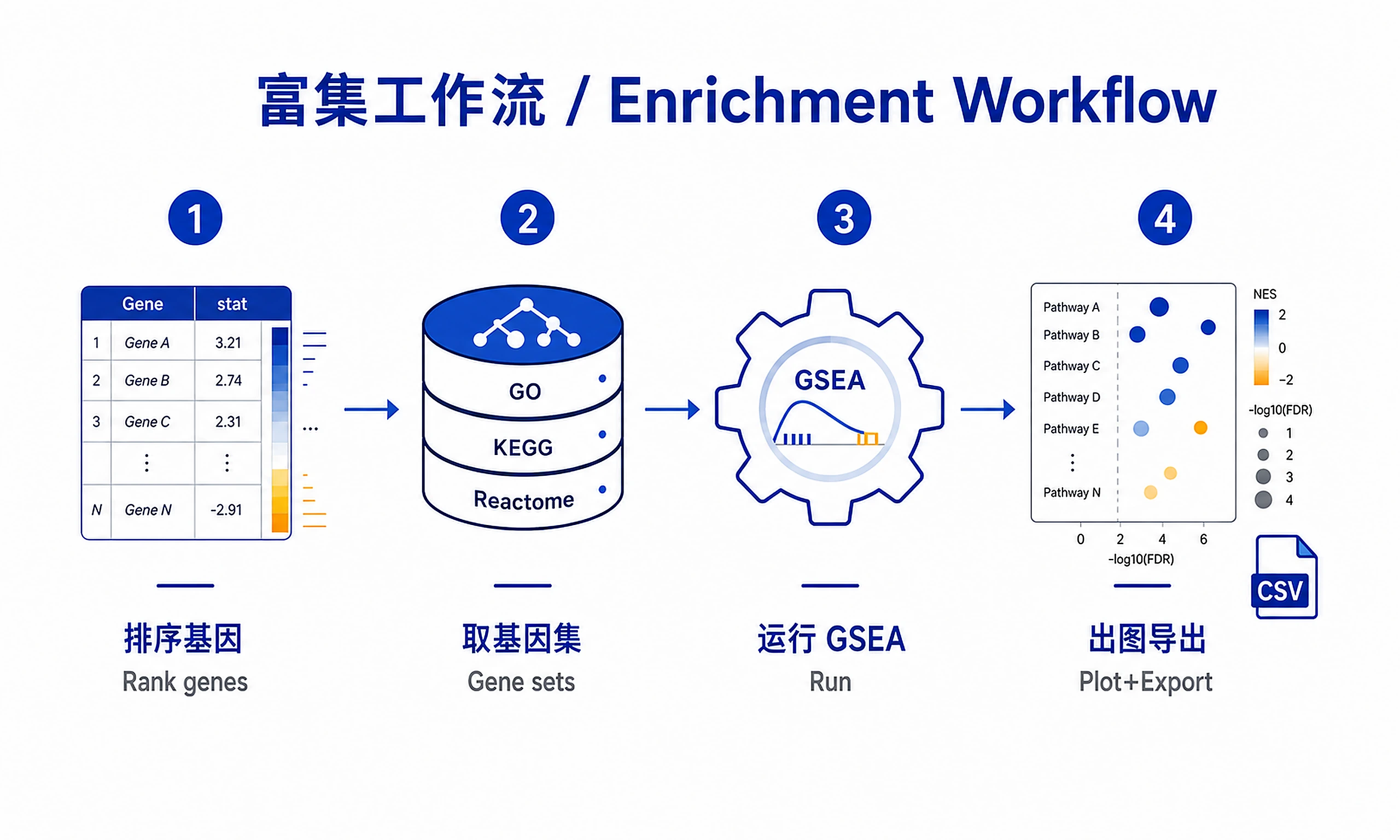
Two complementary methods: GSEA (primary, uses all ranked genes, detects coordinated changes) and ORA (secondary, uses significant gene list, validates GSEA). Default recommendation: Run GSEA unless user specifically requests ORA or has only a gene list (no fold changes).
See references/gsea_ora_comparison.md for detailed method comparison.
Quick Start (Example Data)
Test this skill with real DE results in ~2 minutes:
# Load example DE results from airway dataset (dexamethasone treatment)
source("scripts/load_example_data.R")
de_results <- load_airway_de_results()  # Auto-installs packages (~1-2 min, ~40MB)

# Load required packages and scripts
library(clusterProfiler)
library(msigdbr)
source("scripts/prepare_gene_lists.R")
source("scripts/get_msigdb_genesets.R")
source("scripts/run_gsea.R")
source("scripts/generate_plots.R")
source("scripts/export_results.R")

# Run GSEA workflow
ranked_genes <- create_ranked_list(de_results)
term2gene <- get_msigdb_genesets("human", c("H"))  # Hallmark pathways only for speed
gsea_result <- run_gsea(ranked_genes, term2gene, n_perm = 1000)
generate_all_plots(gsea_result)
export_all(gsea_result, ranked_genes, output_prefix = "quick_test")
What you get:
- Dataset: Human airway smooth muscle cells, dexamethasone treatment vs untreated
- Expected results: ~5-10 significant Hallmark pathways (Inflammatory Response, TNF-alpha signaling, Interferon response)
- Outputs: CSV results, SVG/PNG plots, RDS objects, markdown summary
For your own data: Replace example data loading with your DE results file (see Inputs section).
Installation
# Install Bioconductor packages
if (!require("BiocManager", quietly = TRUE))
    install.packages("BiocManager")

BiocManager::install(c("clusterProfiler", "enrichplot", "org.Hs.eg.db"))

# Install CRAN packages
install.packages(c("msigdbr", "ggplot2", "ggrepel", "dplyr"))
Software Requirements
| Package | Version | License | Commercial Use | Installation |
|---|---|---|---|---|
| clusterProfiler | ≥4.0 | Artistic-2.0 | ✅ Permitted | BiocManager::install("clusterProfiler") |
| enrichplot | ≥1.12 | Artistic-2.0 | ✅ Permitted | BiocManager::install("enrichplot") |
| msigdbr | ≥7.4 | MIT | ✅ Permitted | install.packages("msigdbr") |
| org.Hs.eg.db | Latest | Artistic-2.0 | ✅ Permitted | BiocManager::install("org.Hs.eg.db") |
| org.Mm.eg.db | Latest | Artistic-2.0 | ✅ Permitted | BiocManager::install("org.Mm.eg.db") |
| ggplot2 | ≥3.3 | MIT | ✅ Permitted | install.packages("ggplot2") |
| ggrepel | ≥0.9 | GPL-3 | ✅ Permitted | install.packages("ggrepel") |
| dplyr | ≥1.0 | MIT | ✅ Permitted | install.packages("dplyr") |
Database Licenses
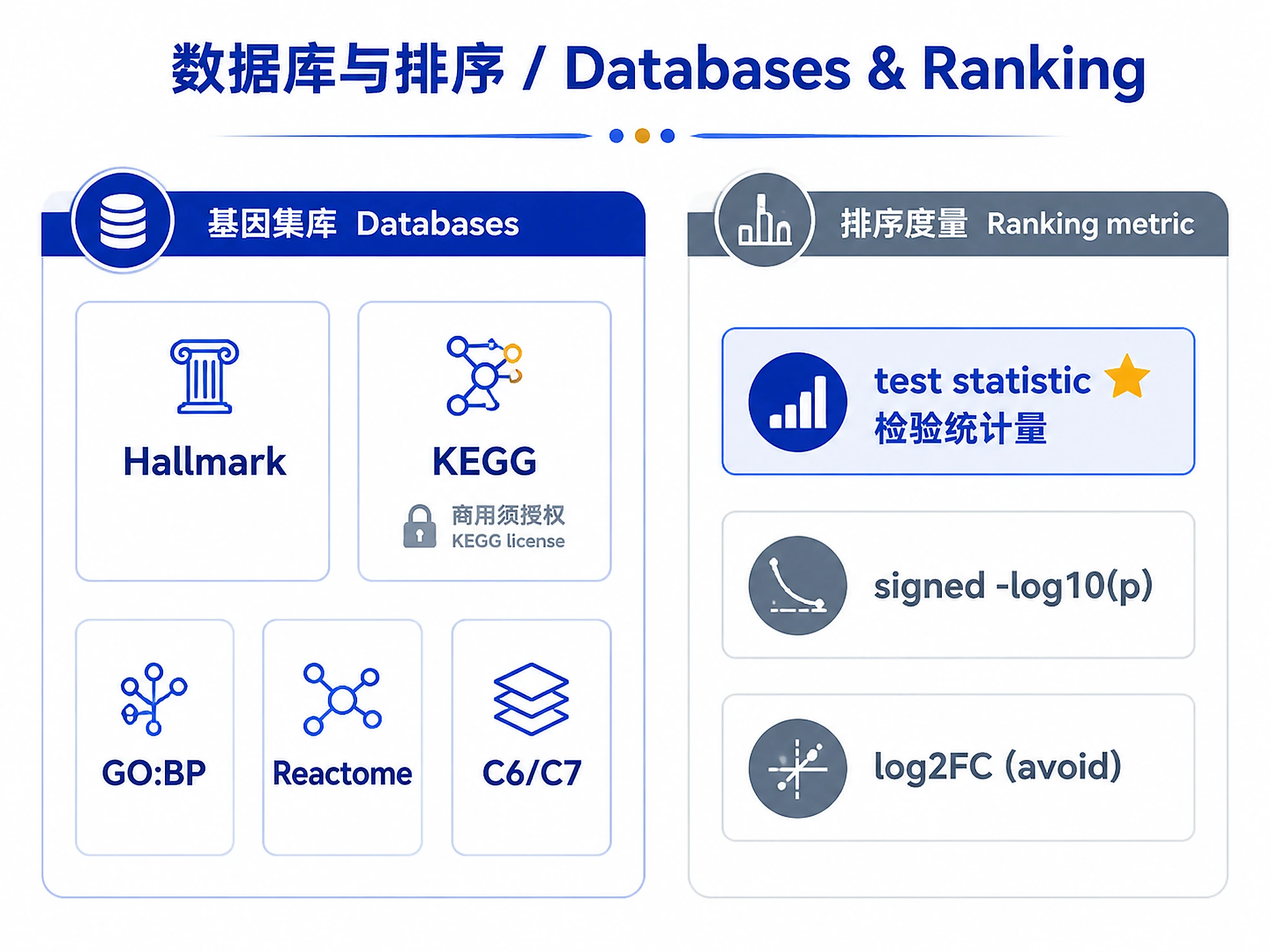
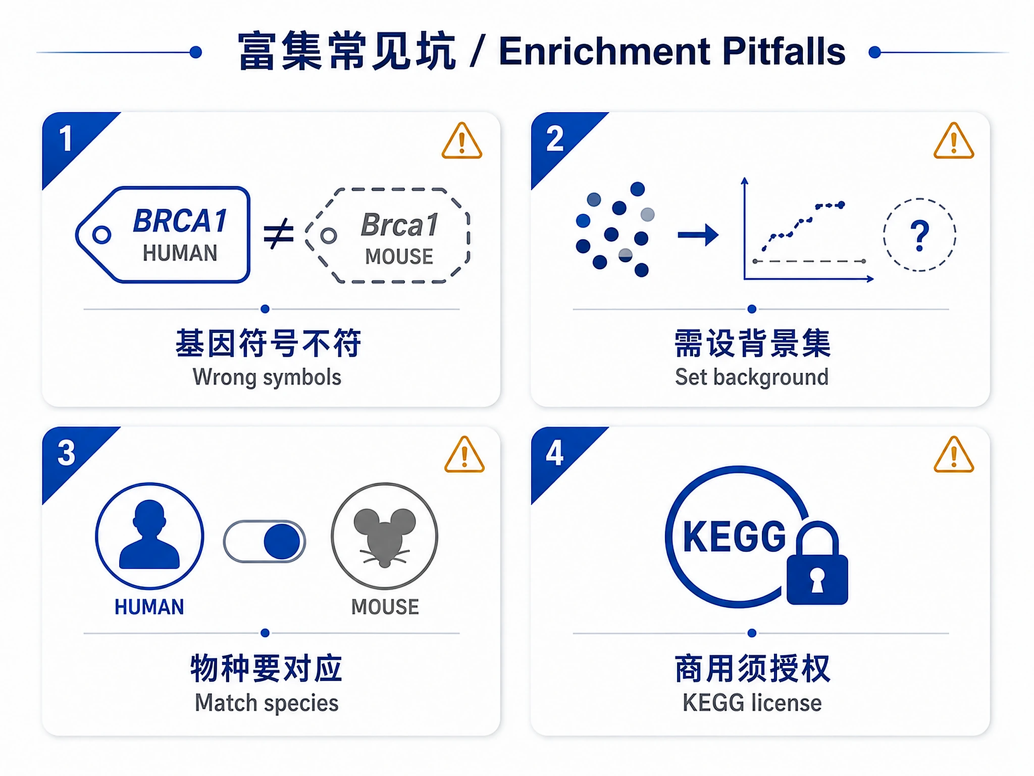
⚠️ KEGG requires commercial license for commercial use. MSigDB and GO use CC-BY 4.0 (commercial use permitted with attribution). For commercial applications, use Hallmark, Reactome, or GO databases, or obtain appropriate KEGG license.
Inputs
Required:
- Differential expression results with:
- Gene identifiers (HGNC symbols preferred)
- Log2 fold change values (for GSEA ranking)
- Adjusted p-values (for ORA filtering)
- Optional: Test statistics for optimal GSEA ranking
Supported DE methods:
- DESeq2 results (padj, log2FoldChange, stat)
- edgeR results (FDR, logFC, logCPM)
- limma results (adj.P.Val, logFC, t)
File formats:
- CSV/TSV files with DE results
- R data frames or result objects
Species support:
- Human (default)
- Mouse
- Other species via custom gene sets
Outputs
Primary results (CSV):
enrichment_gsea_results.csv- All GSEA results (NES, p-value, FDR, leading edge genes)enrichment_ora_up_results.csv- Enriched pathways in upregulated genes (if ORA run)enrichment_ora_down_results.csv- Enriched pathways in downregulated genes (if ORA run)
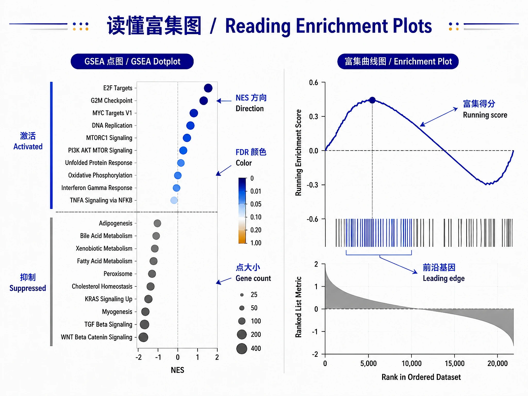
Visualizations (PNG + SVG):
gsea_dotplot.png/.svg- Activated/suppressed pathways visualizationgsea_running_score.png/.svg- Running enrichment score plots for top pathwaysora_up_barplot.png/.svg- Bar plot for upregulated pathways (if ORA run)ora_down_barplot.png/.svg- Bar plot for downregulated pathways (if ORA run)
Analysis objects (RDS):
enrichment_gsea_result.rds- Complete GSEA enrichResult object for downstream use- Load with:
gsea_result <- readRDS('enrichment_gsea_result.rds') - Required for: pathway visualization tools, network analysis, downstream enrichment
enrichment_ora_up_result.rds- ORA enrichResult for upregulated genes (if run)enrichment_ora_down_result.rds- ORA enrichResult for downregulated genes (if run)enrichment_ranked_genes.rds- Ranked gene list used for GSEA- Load with:
ranked_genes <- readRDS('enrichment_ranked_genes.rds')
Summary:
enrichment_summary.md- Text summary of top findings with interpretation
Clarification Questions
Default settings (use unless user specifies otherwise):
- Method: GSEA
- Databases: Hallmark + KEGG
- Species: Human
- ORA thresholds: padj ≤ 0.05, |log2FC| ≥ 1 (only if running ORA)
⚠️ CRITICAL: Always ask question #1 first to check if user has provided input files before proceeding with analysis.
Questions to ask only if ambiguous:
- Input Files (ASK THIS FIRST): - Do you have specific differential expression results file(s) to analyze? - If uploaded: Is this the DE results file (with log2 fold changes and p-values) you'd like to use? - Expected formats: CSV/TSV with gene, log2FoldChange, padj/FDR columns - Or use example data for testing? - Use
source("scripts/load_example_data.R"); de_results <- load_airway_de_results()- Human airway dataset: dexamethasone treatment (~60k genes, ~1-2 min to generate)
- Method: GSEA (default with full DE results), ORA (gene list only), or Both (validation)
- Databases: Hallmark + KEGG (default exploratory), GO:BP (detailed processes), Reactome (alternative to KEGG), C6/C7 (cancer/immunology)
- Species: Human (default) or Mouse
See references/decision-guide.md for detailed decision guidance.
Standard Workflow
🚨 MANDATORY: USE SCRIPTS EXACTLY AS SHOWN - DO NOT WRITE INLINE CODE 🚨
CRITICAL: Use relative paths (scripts/). DO NOT construct absolute paths.
These scripts provide robust, validated enrichment analysis. Use them as-is for standard GSEA workflows.
Step 1 - Load data:
# Load all required scripts
source("scripts/load_de_results.R")
source("scripts/prepare_gene_lists.R")
source("scripts/get_msigdb_genesets.R")
source("scripts/run_gsea.R")
source("scripts/generate_plots.R")
source("scripts/export_results.R")

# Load your DE results
de_results <- load_de_results("your_de_results.csv")  # Replace with your file path

# Prepare inputs
ranked_genes <- create_ranked_list(de_results)
term2gene <- get_msigdb_genesets("human", c("H", "C2:CP:KEGG"))
DO NOT write inline data loading code. Just use the scripts.
Step 2 - Run analysis:
gsea_result <- run_gsea(ranked_genes, term2gene)
DO NOT write inline GSEA code. Just use run_gsea().
Step 3 - Generate visualizations:
generate_all_plots(gsea_result)
DO NOT write inline plotting code (ggsave, dotplot, etc.). Just use generate_all_plots().
The script handles PNG + SVG export with graceful fallback for SVG dependencies.
Step 4 - Export results:
export_all(gsea_result, ranked_genes, output_prefix = "enrichment")
DO NOT write custom export code. Use export_all().
✅ VERIFICATION - You should see:
- After Step 1:
"✓ Data loaded successfully" - After Step 2:
"✓ Analysis completed successfully!" - After Step 3:
"✓ All plots generated successfully!" - After Step 4:
"=== Export Complete ==="
❌ IF YOU DON'T SEE THESE: You wrote inline code. Stop and use the scripts.
⚠️ CRITICAL - DO NOT:
- ❌ Write inline enrichment code → STOP: Use
run_gsea() - ❌ Write inline plotting code (ggsave, dotplot, gseaplot2, etc.) → STOP: Use
generate_all_plots() - ❌ Write custom export code → STOP: Use
export_all() - ❌ Use absolute paths like
/mnt/knowhow/→ use relative pathsscripts/ - ❌ Skip the background parameter in ORA → causes inflated p-values
- ❌ Try to install svglite → script handles SVG fallback automatically
⚠️ IF SCRIPTS FAIL - Script Failure Hierarchy:
- Fix and Retry (90%) - Install missing package, re-run script
- Modify Script (5%) - Edit the script file itself, document changes
- Use as Reference (4%) - Read script, adapt approach, cite source
- Write from Scratch (1%) - Only if genuinely impossible, explain why
NEVER skip directly to writing inline code without trying the script first.
When customization is needed:
- Databases, ranking metrics, thresholds: Read references/decision-guide.md to understand options and adapt to your specific analysis goals
- Complete custom workflow: See references/method-reference.md for step-by-step inline examples (only if user explicitly requests full customization)
- Adding ORA validation: See Pattern 2 in Common Patterns section below
What the scripts provide:
- scripts/load_de_results.R - Standardizes DE results from DESeq2/edgeR/limma
- scripts/load_example_data.R - Loads example datasets for testing
- scripts/prepare_gene_lists.R - Creates ranked lists (GSEA) and filtered lists (ORA)
- scripts/get_msigdb_genesets.R - Retrieves MSigDB gene sets (Hallmark, KEGG, Reactome, GO)
- scripts/run_gsea.R - Runs GSEA with sensible defaults
- scripts/run_ora.R - Runs ORA for up/downregulated genes
- scripts/generate_plots.R - Creates publication-quality PNG + SVG plots with automatic SVG fallback handling
- scripts/export_results.R - Exports CSV results, RDS objects, and markdown summaries
Decision Guide
Key decisions during analysis:
-
Method selection (before analysis): GSEA only (default, full DE results), ORA only (gene list without fold changes), or Both (validation)
-
Database selection (Step 3): Hallmark + KEGG (default exploratory), GO:BP (detailed processes), Reactome (KEGG alternative, commercial-friendly), or C6/C7 (cancer/immunology)
-
Ranking metric (Step 2): Test statistic (best, balances effect + significance), signed -log10(pvalue) (good alternative), or log2FC only (not recommended)
For detailed decision guidance with options and recommendations, see references/decision-guide.md.
Common Patterns
For all patterns and advanced examples, see references/method-reference.md.
Pattern 1: Quick GSEA with Default Settings
# Load required scripts
source("scripts/load_de_results.R")
source("scripts/prepare_gene_lists.R")
source("scripts/get_msigdb_genesets.R")
source("scripts/run_gsea.R")
source("scripts/generate_plots.R")
source("scripts/export_results.R")

# Load, prepare, and run GSEA
de_results <- load_de_results("de_results.csv")
ranked_genes <- create_ranked_list(de_results)
term2gene <- get_msigdb_genesets("human", c("H", "C2:CP:KEGG"))
gsea_result <- run_gsea(ranked_genes, term2gene)
generate_all_plots(gsea_result)
export_all(gsea_result, ranked_genes, output_prefix = "enrichment")
Pattern 2: GSEA + ORA for Validation
# Load required scripts
source("scripts/load_de_results.R")
source("scripts/prepare_gene_lists.R")
source("scripts/get_msigdb_genesets.R")
source("scripts/run_gsea.R")
source("scripts/run_ora.R")
source("scripts/generate_plots.R")
source("scripts/export_results.R")

# Prepare inputs and run both methods
de_results <- load_de_results("de_results.csv")
ranked_genes <- create_ranked_list(de_results)
sig_genes <- filter_significant_genes(de_results)
term2gene <- get_msigdb_genesets("human", c("H", "C2:CP:KEGG"))
gsea_result <- run_gsea(ranked_genes, term2gene)
ora_up <- run_ora(sig_genes$up, term2gene, sig_genes$background, direction = "upregulated")
ora_down <- run_ora(sig_genes$down, term2gene, sig_genes$background, direction = "downregulated")
generate_all_plots(gsea_result)
generate_ora_barplot(ora_up, "Upregulated")
generate_ora_barplot(ora_down, "Downregulated")
export_all(gsea_result, ora_up, ora_down, ranked_genes, output_prefix = "enrichment")
For results interpretation guidance, see references/interpretation_guidelines.md.
Common Errors
| Error | Cause | Solution |
|---|---|---|
| No significant GSEA results | Weak signal, wrong ranking, small gene sets | Try larger databases (GO:BP), verify ranking metric, check DE results quality |
| No significant ORA results | Thresholds too stringent, wrong gene symbols | Relax thresholds (padj < 0.1), verify gene symbols match database |
| Gene symbols not recognized | Wrong species, non-standard IDs | Ensure using official HGNC/MGI symbols, verify species matches database |
| Memory issues with large gene sets | Too many gene sets (e.g., all GO terms) | Reduce max_size parameter, use fewer databases, filter gene sets |
| Slow GSEA execution | High permutations, many gene sets | Reduce n_perm to 1000 for testing, use fewer gene sets |
| Different results between GSEA and ORA | Methods use different information | Normal - GSEA uses all genes, ORA uses cutoff. Check for agreement in top pathways |
| SVG export error "svglite required" | Missing optional dependency | Use generate_all_plots() - it handles fallback automatically. DO NOT try to install svglite manually. |
| svglite dependency conflict | System library version mismatch | Normal - generate_all_plots() falls back to base R svg() device automatically. Both PNG and SVG will be created. |
Suggested Next Steps
After completing functional enrichment analysis:
1. Interpret and Validate Results
Check if enriched pathways align with experimental hypothesis and are biologically coherent. Examine leading edge genes and compare with literature. See references/interpretation_guidelines.md for detailed guidance.
2. Create Additional Visualizations
Generate optional advanced plots: enrichment maps (pathway networks), concept networks (gene-pathway connections), or ridge plots (expression distributions). Use scripts/generate_plots.R.
3. Deep Dive on Key Pathways
Examine leading edge genes in top pathways, check individual gene expression in original DE results, and look up pathway diagrams in KEGG/Reactome databases.
4. Export for Publications
Use CSV results for supplementary tables, SVG plots for figures (300+ DPI), and include enrichment summary in results section. Document database versions, parameters, and software versions in methods.
Related Skills
Prerequisites (run before this skill):
- bulk-rnaseq-counts-to-de-deseq2 - DESeq2 differential expression analysis, generates required DE results
- de-results-to-gene-lists - Filters and annotates DE results, prepares gene lists
Complementary (run alongside):
- de-results-to-plots - Visualize DE results before enrichment to understand expression patterns
Downstream:
- Pathway visualization tools - Coming soon
- Network analysis of enriched pathways - Coming soon
- Integration with other omics data - Coming soon
References
Primary Citations
-
clusterProfiler: Yu G, et al. (2012) clusterProfiler: an R package for comparing biological themes among gene clusters. OMICS. DOI: 10.1089/omi.2011.0118
-
GSEA method: Subramanian A, et al. (2005) Gene set enrichment analysis: A knowledge-based approach for interpreting genome-wide expression profiles. PNAS. DOI: 10.1073/pnas.0506580102
-
MSigDB: Liberzon A, et al. (2015) The Molecular Signatures Database Hallmark Gene Set Collection. Cell Systems. DOI: 10.1016/j.cels.2015.12.004
-
Method benchmarking: Geistlinger L, et al. (2021) Toward a gold standard for benchmarking gene set enrichment analysis. Brief Bioinform. DOI: 10.1093/bib/bbz158
Additional Resources
Detailed documentation:
- references/gsea_ora_comparison.md - Comprehensive GSEA vs ORA comparison
- references/database_guide.md - Gene set database selection guide
- references/interpretation_guidelines.md - Results interpretation guide
- references/gsea_ora_validation_framework.md - Validation framework
Scripts:
- scripts/load_de_results.R - Load and standardize DE results
- scripts/prepare_gene_lists.R - Create ranked/filtered gene lists
- scripts/get_msigdb_genesets.R - Retrieve MSigDB gene sets
- scripts/run_gsea.R - Execute GSEA
- scripts/run_ora.R - Execute ORA
- scripts/generate_plots.R - Visualization functions
- scripts/export_results.R - Export results and summaries
Evaluation:
- assets/eval/ - Evaluation test cases and benchmarking materials
Code preview
scripts/export_results.R
#' Export Enrichment Results
#'
#' Functions to export GSEA and ORA results to CSV files and generate summary reports.


#' Export Results to CSV
#'
#' Saves GSEA and ORA results to CSV files.
#'
#' @param gsea_result enrichResult object from run_gsea()
#' @param ora_up enrichResult object from run_ora() for upregulated genes
#' @param ora_down enrichResult object from run_ora() for downregulated genes
#' @param output_prefix Prefix for output filenames (default: "enrichment")
#' @export
#'
#' @examples
#' export_results(gsea_result, ora_up, ora_down, output_prefix = "my_analysis")

export_results <- function(gsea_result = NULL, ora_up = NULL, ora_down = NULL, output_prefix = "enrichment") {

  message("\n=== Exporting Results ===")

  # GSEA results
  if (!is.null(gsea_result) && nrow(gsea_result@result) > 0) {
    gsea_df <- as.data.frame(gsea_result@result)
    gsea_file <- paste0(output_prefix, "_gsea_results.csv")
    write.csv(gsea_df, gsea_file, row.names = FALSE)
    message(sprintf("  Saved: %s (%d rows)", gsea_file, nrow(gsea_df)))
  }

  # ORA results (up)
  if (!is.null(ora_up) && nrow(ora_up@result) > 0) {
    ora_up_df <- as.data.frame(ora_up@result)
    ora_up_df$direction <- "upregulated"
    ora_up_file <- paste0(output_prefix, "_ora_up_results.csv")
    write.csv(ora_up_df, ora_up_file, row.names = FALSE)
    message(sprintf("  Saved: %s (%d rows)", ora_up_file, nrow(ora_up_df)))
  }

  # ORA results (down)
  if (!is.null(ora_down) && nrow(ora_down@result) > 0) {
    ora_down_df <- as.data.frame(ora_down@result)
    ora_down_df$direction <- "downregulated"
    ora_down_file <- paste0(output_prefix, "_ora_down_results.csv")
    write.csv(ora_down_df, ora_down_file, row.names = FALSE)
    message(sprintf("  Saved: %s (%d rows)", ora_down_file, nrow(ora_down_df)))
  }
}


#' Generate Summary Report
#'
#' Creates a markdown summary of top enrichment findings.
#'
#' @param gsea_result enrichResult object from run_gsea()
#' @param ora_up enrichResult object from run_ora() for upregulated genes
#' @param ora_down enrichResult object from run_ora() for downregulated genes
#' @param output_file Output filename (default: "enrichment_summary.md")
#' @export
#'
#' @examples
#' generate_summary(gsea_result, ora_up, ora_down, output_file = "my_summary.md")

#' Export All Results (export_all wrapper)
#'
#' Comprehensive export function that saves all enrichment results including
#' CSV files, markdown summary, and RDS objects for downstream analysis.
#'
#' This is the recommended function to call for complete result export.
#'
#' @param gsea_result enrichResult object from run_gsea()
#' @param ora_up enrichResult object from run_ora() for upregulated genes (optional)
#' @param ora_down enrichResult object from run_ora() for downregulated genes (optional)
#' @param ranked_genes Named numeric vector of ranked genes (optional, for downstream use)
#' @param output_prefix Prefix for output filenames (default: "enrichment")
#' @export
#'
#' @examples
#' export_all(gsea_result, output_prefix = "my_analysis")
#' export_all(gsea_result, ora_up, ora_down, ranked_genes, output_prefix = "my_analysis")
scripts/generate_plots.R
#' Visualization Functions for Enrichment Results
#'
#' This script contains functions to generate standard plots for GSEA and ORA results.

library(enrichplot)
library(ggplot2)
library(dplyr)

# Try to load svglite for high-quality SVG (optional)
.has_svglite <- requireNamespace("svglite", quietly = TRUE)
if (.has_svglite) {
  library(svglite)
}

#' Save Plot in Both PNG and SVG Formats
#'
#' Internal helper to save plots with graceful fallback for SVG.
#'
#' @param plot ggplot object
#' @param base_path Base filename (without extension)
#' @param width Width in inches
#' @param height Height in inches
#' @param dpi DPI for PNG output
.save_plot <- function(plot, base_path, width = 8, height = 6, dpi = 300) {
  # Always save PNG
  png_path <- sub("\\.(svg|png)$", ".png", base_path)
  ggsave(png_path, plot = plot, width = width, height = height, dpi = dpi, device = "png")
  cat("   Saved:", png_path, "\n")

  # Always try SVG - try ggsave first, fall back to svg() device
  svg_path <- sub("\\.(svg|png)$", ".svg", base_path)
  tryCatch({
    ggsave(svg_path, plot = plot, width = width, height = height, device = "svg")
    cat("   Saved:", svg_path, "\n")
  }, error = function(e) {
    # If ggsave fails, try base R svg() device directly
    tryCatch({
      svg(svg_path, width = width, height = height)
      print(plot)
      dev.off()
      cat("   Saved:", svg_path, "\n")
    }, error = function(e2) {
      cat("   (SVG export failed)\n")
    })
  })
}

#' Generate GSEA Dot Plot (PRIMARY - always generate)
#'
#' Creates a dot plot showing activated vs suppressed pathways from GSEA.
#'
#' @param gsea_result enrichResult object from run_gsea()
#' @param top_n Number of top pathways to show (default: 20)
#' @param output_file Output filename (default: "gsea_dotplot.svg")
#' @return ggplot object
#' @export

generate_gsea_dotplot <- function(gsea_result, top_n = 20, output_file = "gsea_dotplot.svg") {
  if (is.null(gsea_result) || nrow(gsea_result@result) == 0) {
    message("No GSEA results to plot")
    return(NULL)
  }

  p <- dotplot(gsea_result, showCategory = top_n, split = ".sign") +
    facet_grid(~.sign) +
    theme_bw() +
    theme(
      axis.text.y = element_text(size = 8),
      strip.text = element_text(size = 10, face = "bold")
    ) +
    ggtitle("GSEA Results: Activated vs Suppressed Pathways")

  .save_plot(p, output_file, width = 12, height = 8)

  return(p)
}


#' Generate GSEA Running Score Plot
#'
scripts/get_msigdb_genesets.R
#' Get MSigDB Gene Sets
#'
#' Retrieves gene sets from MSigDB for use in enrichment analysis.
#' Supports multiple databases and species.
#'
#' @param species Species name: "human" or "mouse" (default: "human")
#' @param categories Vector of category names to include (default: c("H"))
#'   Options: "H" (Hallmark), "KEGG", "REACTOME", "GO:BP", "GO:MF", "GO:CC"
#' @return Data frame in TERM2GENE format (columns: term, gene)
#' @export
#'
#' @examples
#' # Hallmark gene sets only (default)
#' term2gene <- get_msigdb_genesets(species = "human", categories = c("H"))
#'
#' # Hallmark + KEGG
#' term2gene <- get_msigdb_genesets(species = "human", categories = c("H", "KEGG"))
#'
#' # GO Biological Process
#' term2gene <- get_msigdb_genesets(species = "human", categories = c("GO:BP"))

library(msigdbr)

get_msigdb_genesets <- function(species = "human", categories = c("H")) {
  # Map species
  species_name <- ifelse(species == "human", "Homo sapiens", "Mus musculus")

  # Category mapping (updated for msigdbr >= 10.0.0)
  cat_map <- list(
    "H" = list(collection = "H", subcollection = NULL),           # Hallmark
    "KEGG" = list(collection = "C2", subcollection = "CP:KEGG"),  # KEGG
    "REACTOME" = list(collection = "C2", subcollection = "CP:REACTOME"),
    "GO:BP" = list(collection = "C5", subcollection = "GO:BP"),
    "GO:MF" = list(collection = "C5", subcollection = "GO:MF"),
    "GO:CC" = list(collection = "C5", subcollection = "GO:CC"),
    # Support for old-style subcategory format (e.g., "C2:CP:KEGG")
    "C2:CP:KEGG" = list(collection = "C2", subcollection = "CP:KEGG"),
    "C2:CP:REACTOME" = list(collection = "C2", subcollection = "CP:REACTOME"),
    "C5:GO:BP" = list(collection = "C5", subcollection = "GO:BP"),
    "C5:GO:MF" = list(collection = "C5", subcollection = "GO:MF"),
    "C5:GO:CC" = list(collection = "C5", subcollection = "GO:CC")
  )

  all_genesets <- list()

  for (cat in categories) {
    if (!cat %in% names(cat_map)) {
      warning(sprintf("Unknown category: %s", cat))
      next
    }

    params <- cat_map[[cat]]

    # Use new msigdbr API (collection/subcollection instead of category/subcategory)
    if (is.null(params$subcollection)) {
      msig <- msigdbr(species = species_name, collection = params$collection)
    } else {
      msig <- msigdbr(species = species_name, collection = params$collection,
                      subcollection = params$subcollection)
    }

    # Convert to list format for clusterProfiler
    gs <- split(msig$gene_symbol, msig$gs_name)
    all_genesets <- c(all_genesets, gs)

    message(sprintf("Loaded %d gene sets from %s", length(unique(msig$gs_name)), cat))
  }

  # Convert to TERM2GENE format
  term2gene <- do.call(rbind, lapply(names(all_genesets), function(term) {
    data.frame(term = term, gene = all_genesets[[term]], stringsAsFactors = FALSE)
  }))

  return(term2gene)
}
Companion files
| Type | Path | Bytes |
|---|---|---|
| Text | references/clusterProfiler_GOSemSim.pdf.UNAVAILABLE.txt | 319 |
| Text | references/clusterProfiler_usage_2024.pdf.UNAVAILABLE.txt | 324 |
| Markdown | references/database_guide.md | 8,335 |
| Markdown | references/decision-guide.md | 13,467 |
| Markdown | references/gsea_ora_comparison.md | 6,863 |
| Markdown | references/gsea_ora_validation_framework.md | 13,832 |
| Markdown | references/interpretation_guidelines.md | 11,067 |
| Markdown | references/method-reference.md | 18,684 |
| R | scripts/export_results.R | 7,281 |
| R | scripts/generate_plots.R | 7,358 |
| R | scripts/get_msigdb_genesets.R | 2,884 |
| R | scripts/load_de_results.R | 1,892 |
| R | scripts/load_example_data.R | 7,054 |
| R | scripts/prepare_gene_lists.R | 3,472 |
| R | scripts/run_gsea.R | 1,446 |
| R | scripts/run_ora.R | 1,948 |
| Markdown | SKILL.md | 17,539 |
| JSON | skill.meta.json | 3,366 |