Co-expression Network
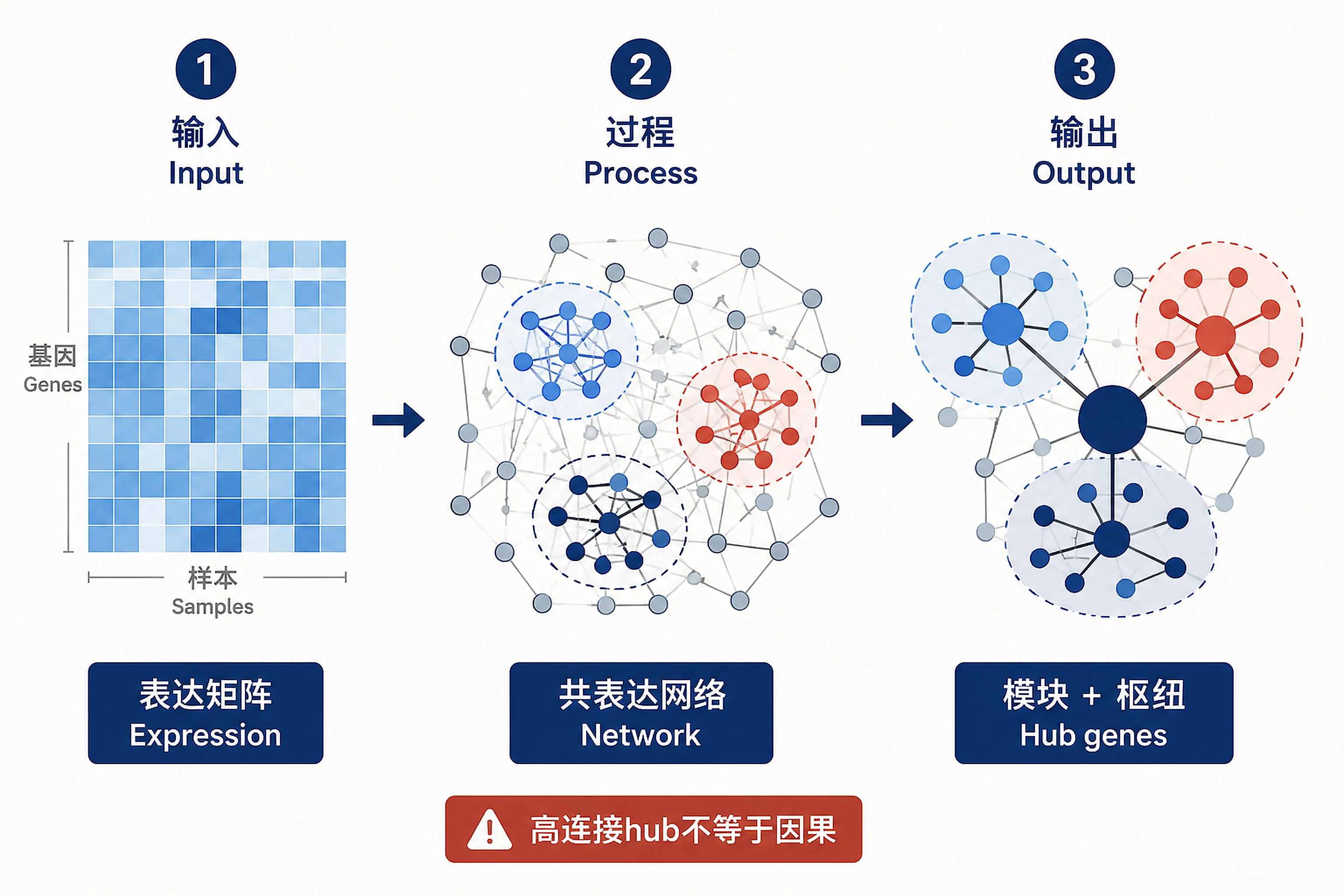
Build a co-expression network; find modules and hub genes.
Overview
Problem. Move from single genes to co-varying modules.
Learning goals
- From gene lists to network thinking
- High connectivity ≠ causation
Figures
Tutorial
Overview
Build weighted gene co-expression networks to identify modules of coordinately expressed genes and discover hub genes that may be key regulators. This workflow uses WGCNA (Weighted Gene Co-expression Network Analysis) to group genes into modules based on their expression patterns across samples, then correlates these modules with experimental conditions or traits.
Key Concept: Unlike single-gene analysis, WGCNA identifies groups of genes that behave similarly across samples, revealing biological pathways and potential regulatory relationships.
Use Cases:
- Identify gene modules associated with experimental conditions
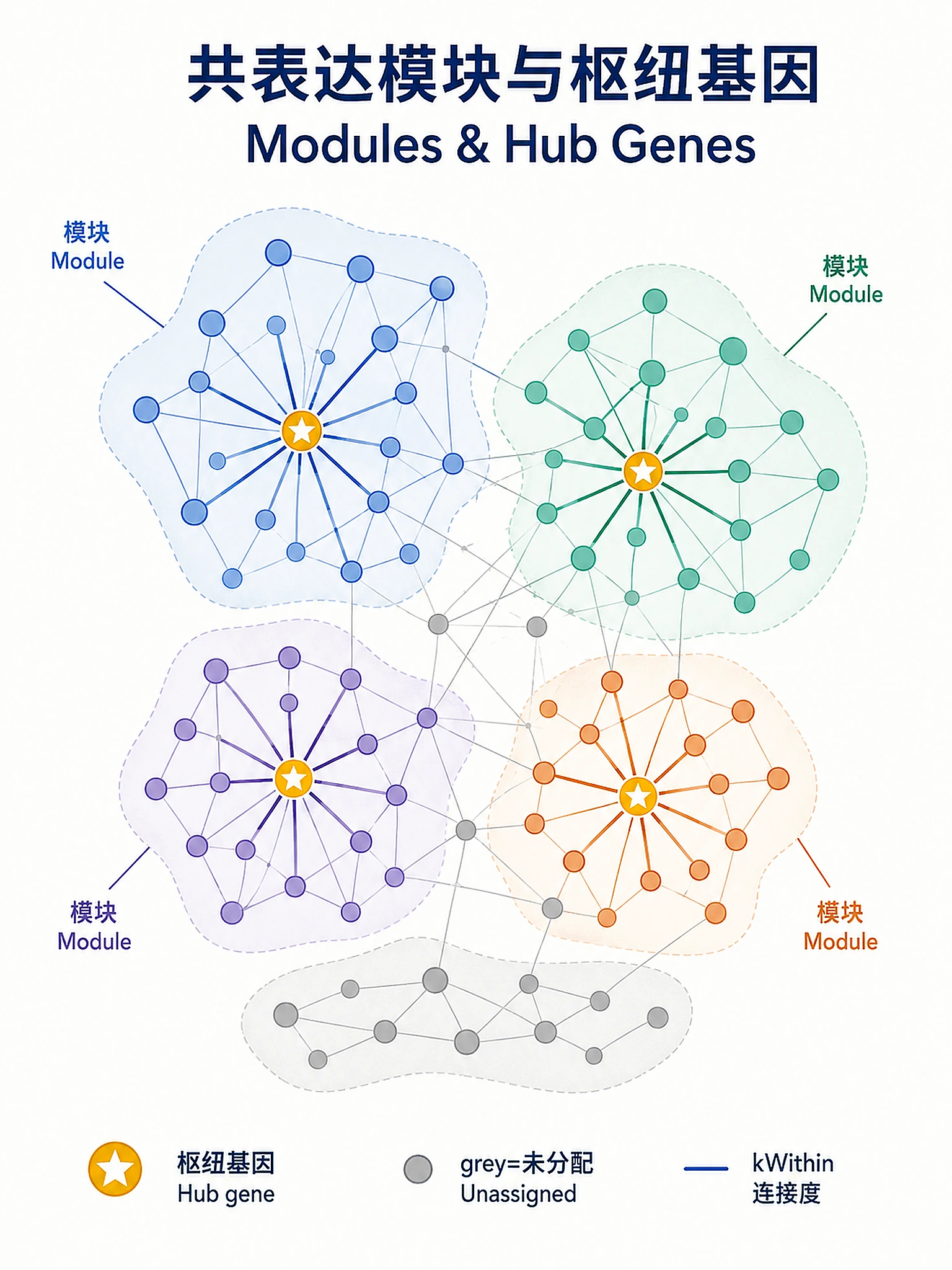
- Discover hub genes (highly connected genes within modules)
- Find genes with similar expression patterns to known genes of interest
- Reduce dimensionality of gene expression data for downstream analysis
- Generate hypotheses about gene function based on co-expression
Default Prompt: "Build a co-expression network to identify gene modules and hub genes from my RNA-seq data"
When to Use This Skill
Use WGCNA when you want to:
- Identify gene modules associated with experimental conditions or phenotypes
- Discover hub genes that are highly connected within modules and may be key regulators
- Find co-expressed genes with similar expression patterns to known genes of interest
- Reduce dimensionality of large gene expression datasets for downstream analysis
- Generate hypotheses about gene function based on co-expression patterns
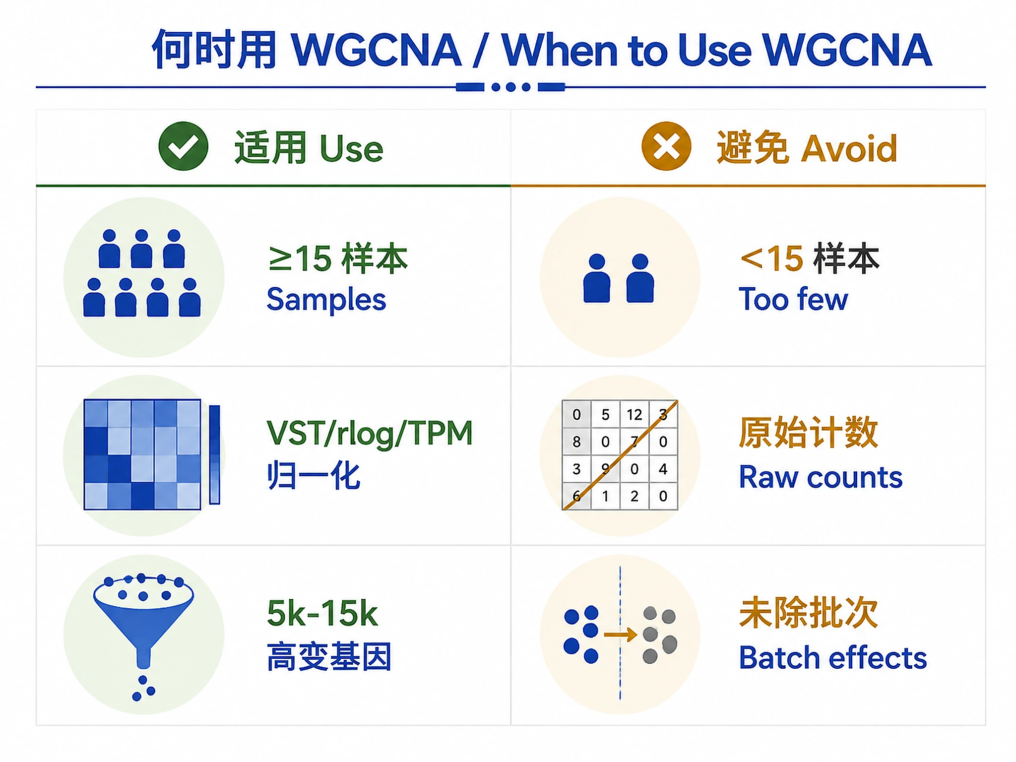
Requirements:
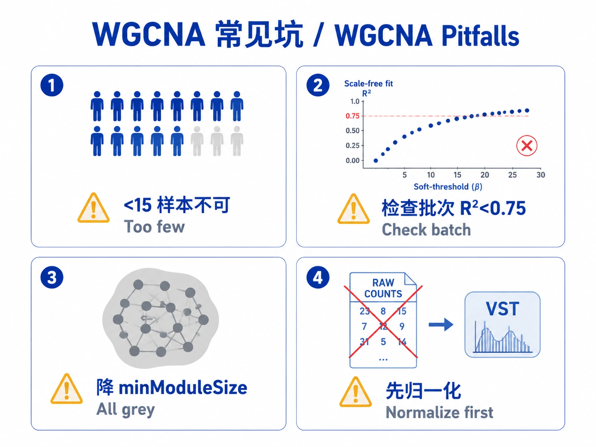
- ≥15 samples (20+ recommended for robust results)
- Normalized expression data (VST, rlog, TPM, or FPKM - NOT raw counts)
- 5,000-15,000 most variable genes
- Batch effects removed or corrected
Not suitable for:
- Small sample sizes (<15 samples) - consider alternative approaches
- Raw count data - normalize first using DESeq2 or similar
- Data with uncorrected batch effects - correct before WGCNA
Installation
Core WGCNA packages:
if (!requireNamespace("BiocManager", quietly = TRUE))
    install.packages("BiocManager")

BiocManager::install("WGCNA")
Visualization packages:
install.packages(c("ggplot2", "ggprism"))
BiocManager::install("ComplexHeatmap")
Enrichment analysis (optional):
BiocManager::install(c("clusterProfiler", "org.Hs.eg.db"))  # Human
# BiocManager::install("org.Mm.eg.db")  # Mouse
# BiocManager::install("org.Rn.eg.db")  # Rat
| Software | Version | License | Commercial Use | Installation |
|---|---|---|---|---|
| WGCNA | ≥1.70 | GPL-2+ | ✅ Permitted | BiocManager::install('WGCNA') |
| ggplot2 | ≥3.3.0 | MIT | ✅ Permitted | install.packages('ggplot2') |
| ComplexHeatmap | ≥2.10.0 | MIT | ✅ Permitted | BiocManager::install('ComplexHeatmap') |
| clusterProfiler | ≥4.0.0 | Artistic-2.0 | ✅ Permitted | BiocManager::install('clusterProfiler') |
Inputs
Required:
- Normalized expression matrix (CSV/TSV): - Rows: Genes, Columns: Samples - Values: VST, rlog, TPM, or FPKM (NOT raw counts) - 5,000-15,000 most variable genes recommended
- Sample metadata (CSV/TSV): - Sample IDs matching expression matrix columns - Traits/conditions for module-trait correlation
Optional:
- Differential expression results (to highlight DEGs)
- Gene annotations for enrichment analysis
Data Requirements:
- ≥15 samples (20+ recommended)
- Batch effects removed or corrected
- No missing values in expression matrix
Outputs
CSV Files:
wgcna_gene_modules.csv- Gene-module assignments with connectivity metricswgcna_hub_genes.csv- Top hub genes per modulewgcna_module_trait_cor.csv- Module-trait correlations with p-valueswgcna_eigengenes.csv- Module eigengene values per samplewgcna_report.md- Summary report with interpretation
Plots (PNG + SVG):
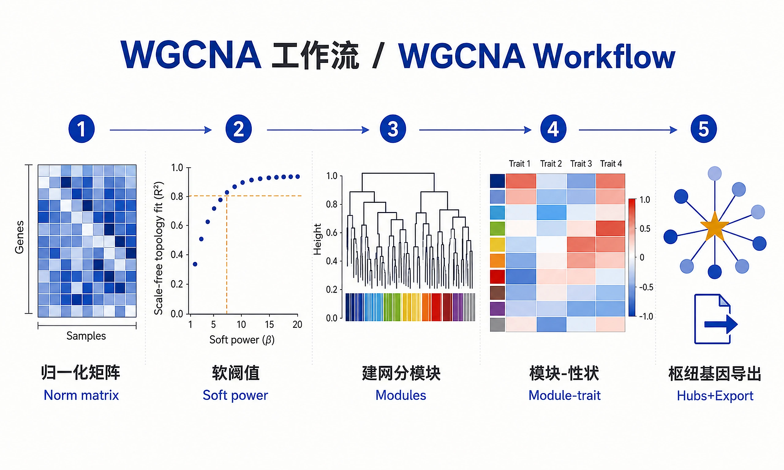
soft_power_selection.png/.svg- Power selection diagnostic plotmodule_dendrogram.png/.svg- Gene dendrogram with module colorsmodule_trait_correlation.png/.svg- Module-trait heatmapeigengene_heatmap.png/.svg- Module eigengene expression patternshub_genes_barplot.png/.svg- Hub genes by connectivity
Analysis Objects (RDS):
wgcna_network.rds- Complete network object from blockwiseModules - Load with:net <- readRDS('wgcna_network.rds')- Required for: module preservation analysis, advanced network visualizationwgcna_module_colors.rds- Module color assignments per gene - Load with:colors <- readRDS('wgcna_module_colors.rds')- Required for: downstream module-specific analyseswgcna_expression_matrix.rds- Filtered expression matrix used for analysis - Load with:expr <- readRDS('wgcna_expression_matrix.rds')- Required for: reanalysis, module preservation testingwgcna_full_results.rds- Complete results object with all components - Load with:results <- readRDS('wgcna_full_results.rds')- Required for: replotting, additional analyses
Key Metrics:
module: Module color assignment (grey = unassigned)kWithin: Intramodular connectivity (higher = more connected)MM: Module membership (correlation with eigengene)hub_score: Combined connectivity metric (MM × kWithin)
Clarification Questions
-
Input Files (ASK THIS FIRST):
- Do you have specific normalized expression data and sample metadata files to analyze?
- If uploaded: Are these the expression matrix and metadata you'd like to analyze?
- Expected formats: CSV or TSV with genes as rows, samples as columns
- Or use example data? Female mouse liver dataset (135 samples, liver tissue, multiple traits)
-
What is your normalized expression data format?
- VST (variance stabilizing transformation) from DESeq2
- rlog (regularized log) from DESeq2
- TPM (transcripts per million)
- FPKM/RPKM
- If unsure or raw counts: normalize first using DESeq2
-
How many samples do you have?
- 15-30 samples (minimum for WGCNA, results may be less robust)
- 30-50 samples (good power for network detection)
- 50+ samples (excellent power, most reliable results)
-
What traits/conditions do you want to correlate with modules?
- Treatment vs control (binary)
- Disease status or phenotype
- Continuous variables (age, dose, time, weight)
- Multiple traits (all will be tested)
-
Gene filtering strategy?
- Top 5,000 most variable genes (default, recommended)
- Top 10,000-15,000 genes (for larger datasets)
- All genes passing expression threshold
- Pre-filtered gene list (e.g., from DE analysis)
Standard Workflow
🚨 MANDATORY: USE SCRIPTS EXACTLY AS SHOWN - DO NOT WRITE INLINE CODE 🚨
Step 1 - Load data:
library(WGCNA)
allowWGCNAThreads()

source("scripts/load_example_data.R")
wgcna_data <- load_example_wgcna_data()
datExpr <- wgcna_data$datExpr
meta <- wgcna_data$meta

# For your own data:
# source("scripts/prepare_wgcna_data.R")
# data <- prepare_wgcna_data("expression.csv", "metadata.csv", top_n_genes = 5000)
# datExpr <- data$datExpr
# meta <- data$meta
Step 2 - Run WGCNA analysis:
source("scripts/wgcna_workflow.R")
results <- run_wgcna_analysis(
  datExpr,
  meta,
  traits = c("weight_g", "Glucose_mg_dl"),  # Adjust to your traits
  organism = "mouse"  # or "human", "rat", or NULL to skip enrichment
)
DO NOT write inline WGCNA code. Just source the script.
Step 3 - Generate visualizations:
source("scripts/plot_all_wgcna.R")
plot_all_wgcna(results, output_dir = "wgcna_results")
DO NOT write inline plotting code (png, svg, plotDendroAndColors, etc.). Just use the script.
The script handles PNG + SVG export with graceful fallback for SVG dependencies.
Step 4 - Export results:
source("scripts/export_wgcna_results.R")
export_all(results, output_dir = "wgcna_results")
DO NOT write custom export code. Use export_all().
✅ VERIFICATION - You should see:
- After Step 1:
"✓ Successfully loaded female mouse liver dataset" - After Step 2:
"✓ WGCNA analysis completed successfully!" - After Step 3:
"✓ All WGCNA plots generated successfully!" - After Step 4:
"=== Export Complete ==="
⚠️ CRITICAL - DO NOT:
- ❌ Write inline WGCNA code → STOP: Use
source("scripts/wgcna_workflow.R") - ❌ Write inline plotting code (png, svg, plotDendroAndColors, etc.) → STOP: Use
plot_all_wgcna() - ❌ Write custom export code → STOP: Use
export_all() - ❌ Try to install svglite → script handles SVG fallback automatically
- ❌ Use absolute paths like
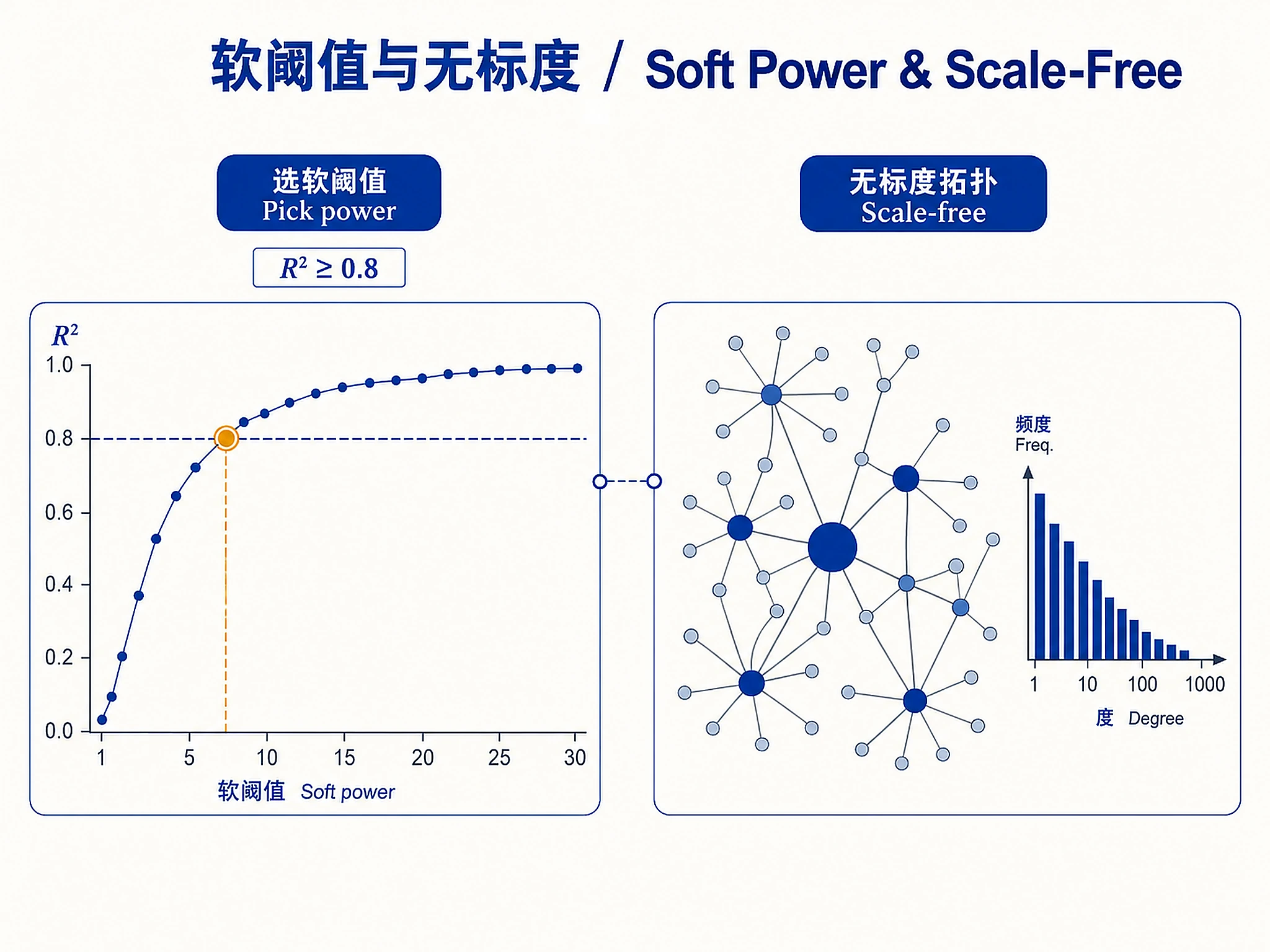
/mnt/knowhow/→ use relative pathsscripts/ - ❌ Skip soft power selection → required for scale-free topology
- ❌ Use raw counts → normalize first with DESeq2 VST or rlog
⚠️ IF SCRIPTS FAIL - Script Failure Hierarchy:
- Fix and Retry (90%) - Install missing package, re-run script
- Modify Script (5%) - Edit the script file itself, document changes
- Use as Reference (4%) - Read script, adapt approach, cite source
- Write from Scratch (1%) - Only if genuinely impossible, explain why
NEVER skip directly to writing inline code without trying the script first.
What the scripts provide:
- scripts/load_example_data.R - Auto-fetch tutorial data (~135 samples)
- scripts/prepare_wgcna_data.R - Load and filter your data
- scripts/wgcna_workflow.R - Complete WGCNA analysis (power selection, network building, module-trait correlation, hub genes, enrichment)
- scripts/plot_all_wgcna.R - All publication-quality plots (PNG + SVG)
- scripts/plotting_helpers.R - Plot saving functions with automatic SVG fallback handling
- scripts/export_wgcna_results.R - Export results and analysis objects
Parameter Customization
When customization is needed:
- Soft power selection: Read references/parameter-tuning-guide.md to understand how to choose appropriate power values for your data
- Module detection parameters: See references/parameter-tuning-guide.md#module-detection for guidance on min_module_size and merge_cut_height
- Complete custom workflow: Read references/wgcna-reference.md for detailed code examples with explanations (only if you need full control)
Common Issues
| Issue | Cause | Solution |
|---|---|---|
| Too few samples error | <15 samples | WGCNA requires ≥15 samples; combine replicates or use alternative methods |
| Scale-free R² never exceeds 0.75 | Batch effects or poor data quality | Check for batch effects; try different normalization; inspect PCA |
| All genes assigned to grey module | minModuleSize too large or poor gene filtering | Lower minModuleSize to 20-30; increase top_n_genes to 10,000-15,000 |
| No significant module-trait correlations | Weak biological signal or incorrect traits | Check trait coding (numeric for continuous, 0/1 for binary); try more samples |
| Soft power recommended is very high (>20) | Data not suitable for scale-free network | Check normalization; consider signed vs unsigned network |
| Hub gene identification fails | Module colors not provided correctly | Ensure module_colors matches gene order in datExpr |
| Enrichment analysis returns no results | Wrong organism or gene ID format | Verify organism parameter matches data; convert gene IDs if needed |
| Memory errors during network construction | Too many genes | Reduce to 5,000-10,000 most variable genes; increase RAM |
Interpretation Guidelines
Module colors:
- Each color = distinct co-expression module
- Grey = genes not assigned to any module
- Larger modules may represent broader biological processes
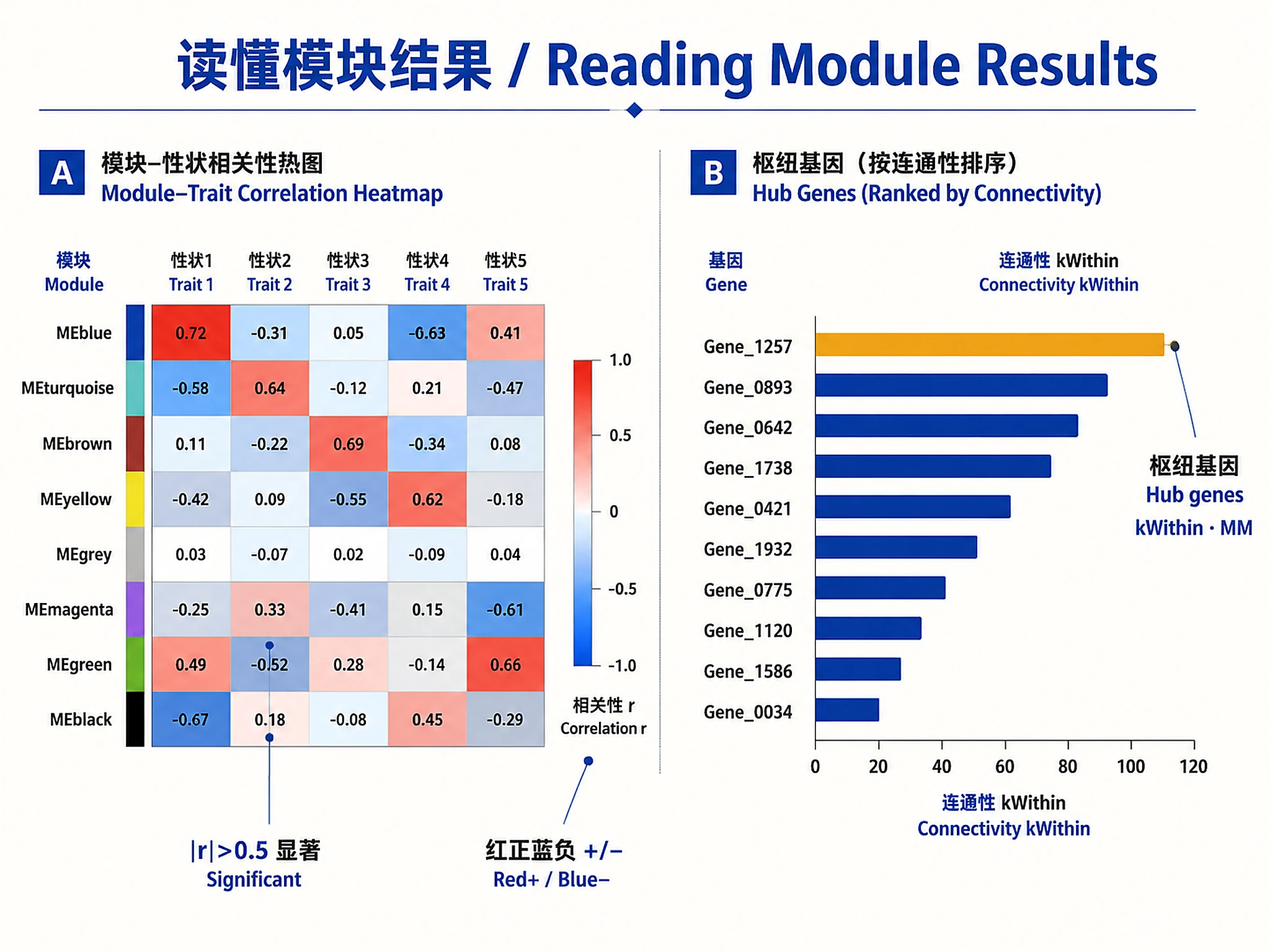
Hub genes:
- High
kWithin= highly connected within module - High
MM= strong correlation with module eigengene - Hub genes are candidates for experimental validation
Module-trait correlations:
- |r| > 0.5 and p < 0.05 = significant association
- Positive correlation = module genes increase with trait
- Negative correlation = module genes decrease with trait
- Focus on modules with strongest associations
Suggested Next Steps
After identifying modules and hub genes:
- Functional validation - Validate hub genes experimentally (qPCR, knockdown, overexpression)
- Enrichment analysis - Test modules for GO/KEGG enrichment to understand biological processes
- Compare with DE results - Overlay DE genes on network to see which modules are enriched
- Network visualization - Export to Cytoscape for detailed network visualization
- Cross-dataset validation - Test module preservation in independent datasets
Related Skills
- bulk-rnaseq-counts-to-de-deseq2 - Normalize counts and perform differential expression analysis (run before WGCNA)
- de-results-to-gene-lists - Extract gene lists from DE results to overlay on network
- functional-enrichment-from-degs - Perform GO/KEGG enrichment on modules
References
Documentation:
- WGCNA Best Practices Guide - Comprehensive guide on data preparation, QC, and troubleshooting
- Parameter Tuning Guide - Detailed parameter selection guidance
- WGCNA Reference - Complete code examples with explanations
- Troubleshooting Guide - Common errors and solutions
Example Data:
- Example Datasets - Public datasets for WGCNA analysis
Key Papers:
- Key WGCNA Papers - Essential publications
- Langfelder & Horvath (2008). WGCNA: an R package for weighted correlation network analysis. BMC Bioinformatics. doi:10.1186/1471-2105-9-559
- Zhang & Horvath (2005). A general framework for weighted gene co-expression network analysis. Statistical Applications in Genetics and Molecular Biology. doi:10.2202/1544-6115.1128
Code preview
scripts/build_network.R
# Build co-expression network and detect modules

library(WGCNA)

#' Build co-expression network and detect modules
#'
#' @param datExpr Expression matrix (samples x genes)
#' @param power Soft-thresholding power
#' @param min_module_size Minimum genes per module
#' @param merge_cut_height Height for merging similar modules
#' @return List containing network object, module colors, and module labels
build_network <- function(datExpr, power, min_module_size = 30, merge_cut_height = 0.25) {

  cat("Building network with power =", power, "\n")

  # One-step network construction and module detection
  net <- blockwiseModules(
    datExpr,
    power = power,
    TOMType = "signed",
    networkType = "signed",
    minModuleSize = min_module_size,
    reassignThreshold = 0,
    mergeCutHeight = merge_cut_height,
    numericLabels = TRUE,
    pamRespectsDendro = FALSE,
    saveTOMs = FALSE,
    verbose = 3
  )

  # Convert numeric labels to colors
  module_colors <- labels2colors(net$colors)

  cat("\nModule detection complete:\n")
  cat("Number of modules:", length(unique(module_colors)) - 1, "(excluding grey/unassigned)\n")
  print(table(module_colors))

  return(list(
    net = net,
    module_colors = module_colors,
    module_labels = net$colors
  ))
}
scripts/correlate_modules_traits.R
# Correlate module eigengenes with sample traits

library(WGCNA)
library(ComplexHeatmap)
library(circlize)

#' Correlate module eigengenes with sample traits
#'
#' @param datExpr Expression matrix
#' @param module_colors Module color assignments
#' @param traits Data frame of sample traits (numeric)
#' @param output_file Path to save heatmap
#' @return List with module eigengenes, correlations, and p-values
correlate_modules_traits <- function(datExpr, module_colors, traits,
                                      output_file = "module_trait_correlation.svg") {

  # Calculate module eigengenes
  MEs <- moduleEigengenes(datExpr, colors = module_colors)$eigengenes
  MEs <- orderMEs(MEs)

  # Convert traits to numeric if needed
  traits_numeric <- data.frame(lapply(traits, function(x) {
    if (is.factor(x) || is.character(x)) {
      as.numeric(as.factor(x))
    } else {
      as.numeric(x)
    }
  }))
  rownames(traits_numeric) <- rownames(traits)

  # Calculate correlations
  module_trait_cor <- cor(MEs, traits_numeric, use = "pairwise.complete.obs")
  module_trait_pval <- corPvalueStudent(module_trait_cor, nrow(datExpr))

  # Create text matrix for heatmap (correlation and p-value)
  text_matrix <- matrix(
    paste0(signif(module_trait_cor, 2), "\n(", signif(module_trait_pval, 1), ")"),
    nrow = nrow(module_trait_cor),
    ncol = ncol(module_trait_cor)
  )

  # Create color function
  col_fun <- colorRamp2(c(-1, 0, 1), c("blue", "white", "red"))

  # Create heatmap with ComplexHeatmap
  ht <- Heatmap(
    module_trait_cor,
    name = "Correlation",
    col = col_fun,
    cluster_rows = FALSE,
    cluster_columns = FALSE,
    show_row_names = TRUE,
    show_column_names = TRUE,
    row_names_side = "left",
    column_names_side = "bottom",
    column_title = "Module-Trait Relationships",
    cell_fun = function(j, i, x, y, width, height, fill) {
      grid.text(text_matrix[i, j], x, y, gp = gpar(fontsize = 8))
    },
    heatmap_legend_param = list(
      title = "Correlation",
      at = c(-1, -0.5, 0, 0.5, 1)
    ),
    width = unit(max(8, ncol(traits) * 1.5), "cm"),
    height = unit(max(8, nrow(module_trait_cor) * 0.5), "cm")
  )

  # Save to file
  svg(output_file, width = max(8, ncol(traits) * 1.5), height = max(8, nrow(module_trait_cor) * 0.4))
  draw(ht)
  dev.off()

  cat("Saved:", output_file, "\n")

  # Return results
  results <- data.frame(
    module = rownames(module_trait_cor),
    stringsAsFactors = FALSE
  )
scripts/export_wgcna_results.R
# Export all WGCNA results

library(WGCNA)

#' Export all WGCNA results (including RDS objects for downstream skills)
#'
#' @param results Results object from run_wgcna_analysis()
#' @param output_dir Directory to save results (default: "wgcna_results")
#' @param output_prefix Prefix for output files (default: "wgcna")
export_all <- function(results, output_dir = "wgcna_results", output_prefix = "wgcna") {

  cat("\n=== Exporting WGCNA Results ===\n\n")

  # Create output directory if needed
  if (!dir.exists(output_dir)) {
    dir.create(output_dir, recursive = TRUE)
  }

  # Extract components from results
  gene_info <- results$hub_results$gene_info
  hub_genes <- results$hub_results$hub_genes
  trait_results <- results$trait_results

  # 1. Export gene-module assignments
  csv_path <- file.path(output_dir, paste0(output_prefix, "_gene_modules.csv"))
  write.csv(gene_info, csv_path, row.names = FALSE)
  cat("  Saved:", csv_path, "\n")

  # 2. Export hub genes
  hub_df <- do.call(rbind, lapply(names(hub_genes), function(mod) {
    df <- hub_genes[[mod]]
    df$module <- mod
    df
  }))
  csv_path <- file.path(output_dir, paste0(output_prefix, "_hub_genes.csv"))
  write.csv(hub_df, csv_path, row.names = FALSE)
  cat("  Saved:", csv_path, "\n")

  # 3. Export module-trait correlations
  csv_path <- file.path(output_dir, paste0(output_prefix, "_module_trait_cor.csv"))
  write.csv(trait_results$results, csv_path, row.names = FALSE)
  cat("  Saved:", csv_path, "\n")

  # 4. Export module eigengenes
  csv_path <- file.path(output_dir, paste0(output_prefix, "_eigengenes.csv"))
  write.csv(trait_results$MEs, csv_path)
  cat("  Saved:", csv_path, "\n")

  # 5. Save analysis objects as RDS for downstream skills (CRITICAL)
  cat("\n  Saving analysis objects for downstream use:\n")

  rds_path <- file.path(output_dir, paste0(output_prefix, "_network.rds"))
  saveRDS(results$network, rds_path)
  cat("    • wgcna_network.rds\n")
  cat("      (Load with: net <- readRDS('", basename(rds_path), "'))\n", sep = "")

  rds_path <- file.path(output_dir, paste0(output_prefix, "_module_colors.rds"))
  saveRDS(results$module_colors, rds_path)
  cat("    • wgcna_module_colors.rds\n")
  cat("      (Load with: colors <- readRDS('", basename(rds_path), "'))\n", sep = "")

  rds_path <- file.path(output_dir, paste0(output_prefix, "_expression_matrix.rds"))
  saveRDS(results$datExpr, rds_path)
  cat("    • wgcna_expression_matrix.rds\n")
  cat("      (Load with: expr <- readRDS('", basename(rds_path), "'))\n", sep = "")

  rds_path <- file.path(output_dir, paste0(output_prefix, "_full_results.rds"))
  saveRDS(results, rds_path)
  cat("    • wgcna_full_results.rds (complete results object)\n")
  cat("      (Load with: results <- readRDS('", basename(rds_path), "'))\n", sep = "")

  # 6. Create summary report
  cat("\n  Creating summary report...\n")
  summary_lines <- c(
    "# WGCNA Co-expression Network Analysis Summary\n",
    paste("**Total genes analyzed:**", nrow(gene_info)),
    paste("**Total samples:**", nrow(trait_results$MEs)),
    paste("**Number of modules:**", length(unique(gene_info$module)) - 1, "(excluding grey)\n"),
    "## Module Sizes"
  )
Companion files
| Type | Path | Bytes |
|---|---|---|
| Text | references/2008_WGCNA an R package for weighted correlation network analysis.pdf.UNAVAILABLE.txt | 391 |
| Text | references/2021_WGCNA Gene Correlation Network Analysis - Bioinformatics Workbook.pdf.UNAVAILABLE.txt | 401 |
| Markdown | references/parameter-tuning-guide.md | 15,005 |
| Markdown | references/troubleshooting.md | 10,604 |
| Markdown | references/wgcna-best-practices.md | 15,201 |
| Markdown | references/wgcna-reference.md | 14,644 |
| R | scripts/build_network.R | 1,269 |
| R | scripts/correlate_modules_traits.R | 2,786 |
| R | scripts/export_wgcna_results.R | 4,480 |
| R | scripts/identify_hub_genes.R | 1,958 |
| R | scripts/load_example_data.R | 7,444 |
| R | scripts/module_enrichment.R | 5,033 |
| R | scripts/pick_soft_power.R | 2,452 |
| R | scripts/plot_all_wgcna.R | 4,065 |
| R | scripts/plot_eigengene_heatmap.R | 1,801 |
| R | scripts/plot_hub_genes.R | 2,325 |
| R | scripts/plot_module_dendrogram.R | 1,408 |
| R | scripts/plotting_helpers.R | 2,930 |
| R | scripts/prepare_wgcna_data.R | 2,548 |
| R | scripts/wgcna_workflow.R | 3,586 |
| Markdown | SKILL.md | 13,975 |
| JSON | skill.meta.json | 4,083 |