Spatial Transcriptomics
Clustering and spatial analysis that keeps tissue location.
Overview
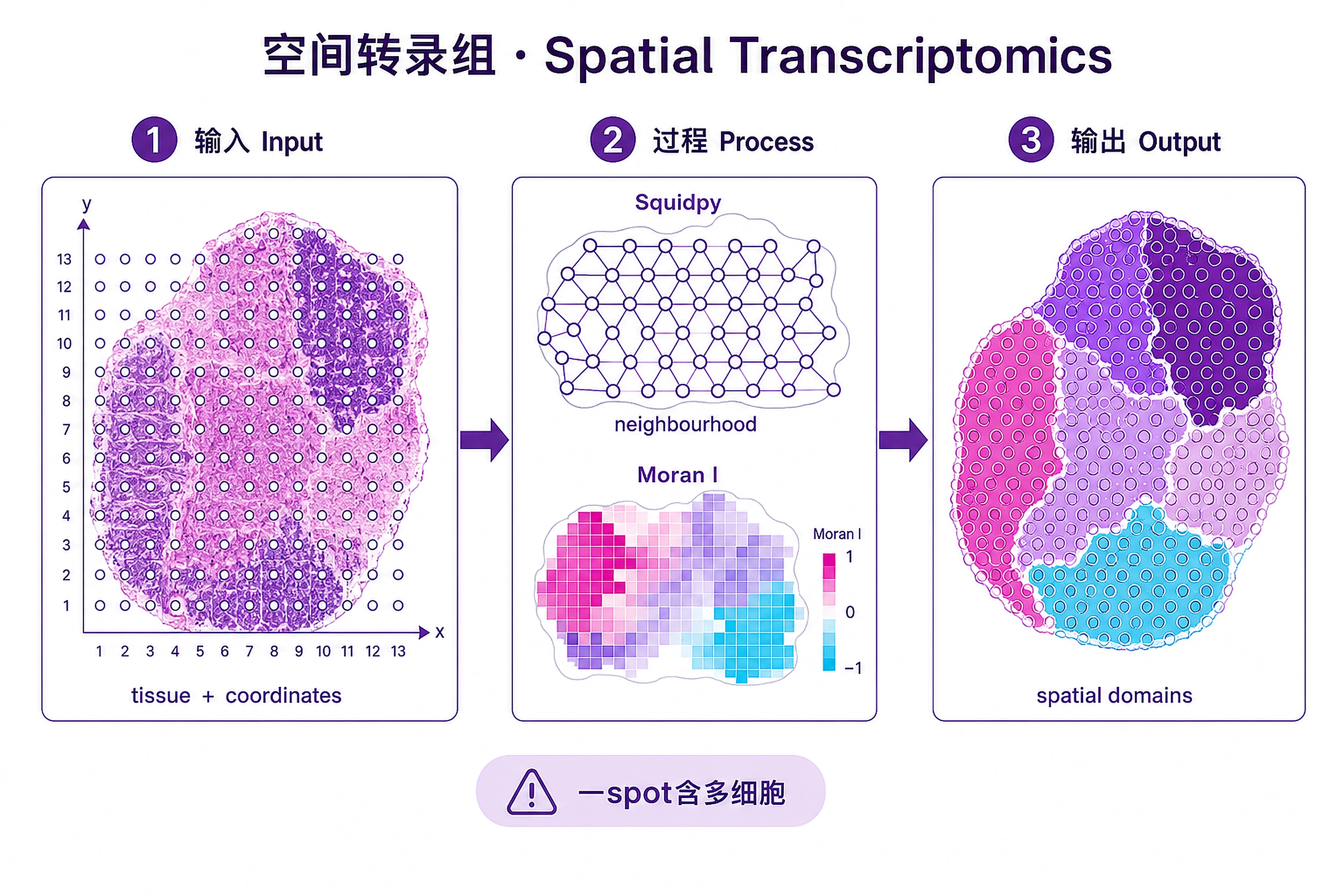
Problem. Not just what cells express, but where.
Learning goals
- Location adds a dimension; Moran's I
- A spot often holds several cells
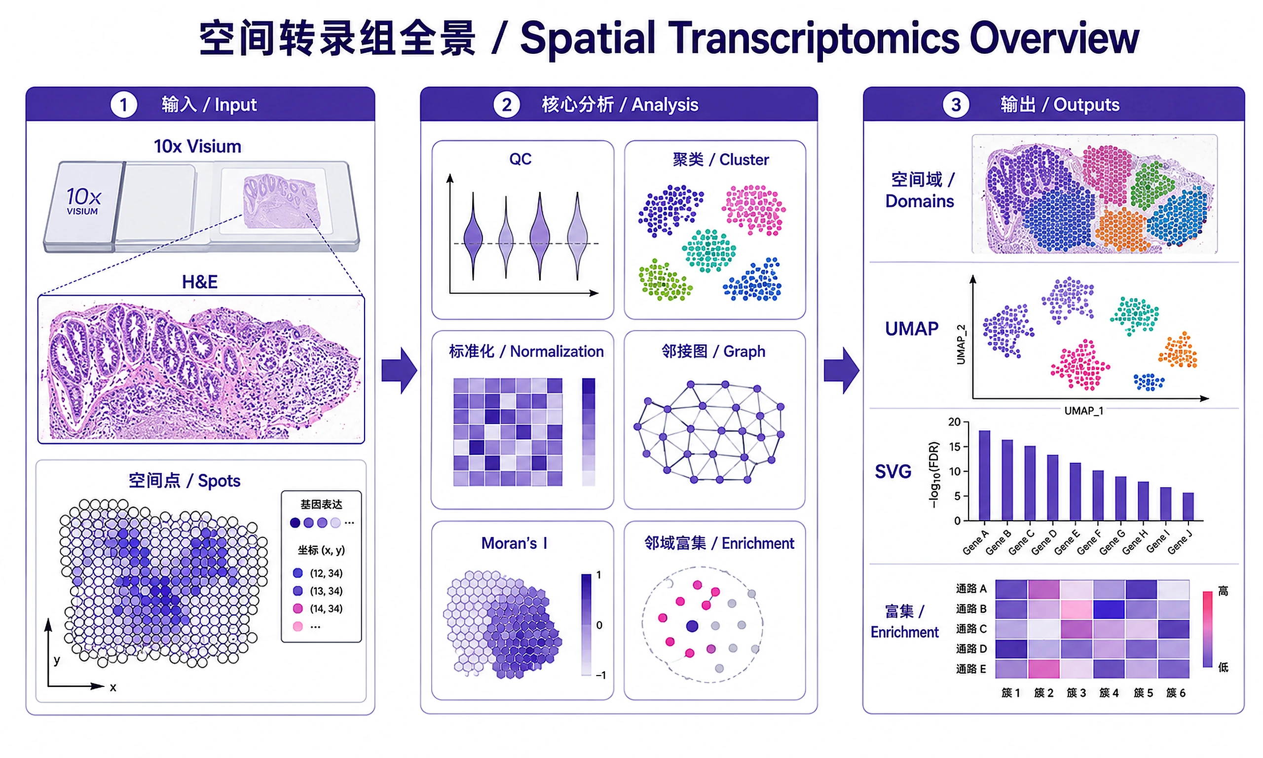
Figures
Tutorial
When to Use This Skill
- You have 10x Visium spatial gene expression data (with or without H&E image)
- You want to identify spatially variable genes across a tissue section
- You want to discover spatial tissue domains via clustering
- You want to quantify neighborhood enrichment between cell clusters
- You want to analyze co-occurrence patterns of cell types across distances
- Input is Space Ranger output,
.h5ad, or.h5file
Not for: Single-molecule FISH (MERFISH/Xenium), Slide-seq, or single-cell RNA-seq without spatial coordinates. For scRNA-seq, use scrnaseq-scanpy-core-analysis.
Installation
pip install squidpy scanpy anndata scikit-misc plotnine plotnine-prism seaborn matplotlib numpy pandas scikit-learn
| Package | Version | License | Commercial Use | Installation |
|---|---|---|---|---|
| squidpy | ≥1.4 | BSD-3-Clause | ✅ Permitted | pip install squidpy |
| scanpy | ≥1.9 | BSD-3-Clause | ✅ Permitted | pip install scanpy |
| anndata | ≥0.8 | BSD-3-Clause | ✅ Permitted | pip install anndata |
| plotnine | ≥0.12 | MIT | ✅ Permitted | pip install plotnine |
| plotnine-prism | ≥0.2 | MIT | ✅ Permitted | pip install plotnine-prism |
| seaborn | ≥0.11 | BSD-3-Clause | ✅ Permitted | pip install seaborn |
| matplotlib | ≥3.5 | PSF | ✅ Permitted | pip install matplotlib |
| scikit-learn | ≥1.0 | BSD-3-Clause | ✅ Permitted | pip install scikit-learn |
| scikit-misc | ≥0.1 | BSD-3-Clause | ✅ Permitted | pip install scikit-misc |
| numpy | ≥1.21 | BSD-3-Clause | ✅ Permitted | pip install numpy |
| pandas | ≥1.3 | BSD-3-Clause | ✅ Permitted | pip install pandas |
License Compliance: All packages use permissive licenses (BSD, MIT, PSF) that permit commercial use in AI agent applications.
Inputs
| Input | Format | Description |
|---|---|---|
| Visium data | .h5ad, .h5, or Space Ranger directory |
Gene expression + spatial coordinates |
| H&E image | Embedded in above | Tissue histology (optional, enhances spatial plots) |
Built-in example: V1_Human_Heart from 10x Genomics (~4,247 spots, ~33,538 genes, includes H&E image).
Outputs
Analysis objects:
adata_processed.h5ad— Complete processed AnnData for downstream use- Load with:
adata = sc.read_h5ad('adata_processed.h5ad') - Contains: clusters, embeddings, SVG results, spatial graph
Tables (CSV):
spatially_variable_genes.csv— SVGs ranked by Moran's I with FDRcluster_assignments.csv— Spot barcodes + Leiden cluster + spatial coordinatesneighborhood_enrichment.csv— Cluster-cluster enrichment z-scoresspot_metadata.csv— All spot-level QC and annotation metadataanalysis_summary.txt— Human-readable report
Plots (PNG + SVG):
qc_violins— QC metric distributionsspatial_clusters— Leiden clusters overlaid on tissuespatial_markers— Selected marker gene expression on tissueumap_clusters— UMAP embedding colored by clusterneighborhood_enrichment— Cluster enrichment heatmapco_occurrence— Co-occurrence probability vs distancetop_svgs— Bar chart of top spatially variable genesspatial_svg_[GENE]— Spatial expression of top SVG
Clarification Questions
ALWAYS ask Question 1 FIRST:
1. Input Files (ASK THIS FIRST):
- Do you have Visium data files to analyze?
- Supported formats:
.h5ad,.h5, or Space Ranger output directory - Or use example data? V1_Human_Heart from 10x Genomics (human cardiac tissue, ~4K spots)
🚨 IF EXAMPLE DATA SELECTED: All parameters are pre-configured. Skip remaining questions. Proceed directly to Step 1.
2. Analysis Parameters (ONLY if user provides own data):
- Clustering resolution?
- a) 0.5 (fewer, broader clusters)
- b) 0.8 (standard — recommended)
- c) 1.2 (more, finer clusters)
- Mitochondrial threshold?
- a) 50% (recommended for cardiac/muscle tissue — high MT is normal)
- b) 20% (standard for most tissues)
- c) 30% (moderate)
3. Marker Genes (ONLY if user provides own data):
- Which marker genes to highlight in spatial plots?
- Provide a list or use tissue-appropriate defaults
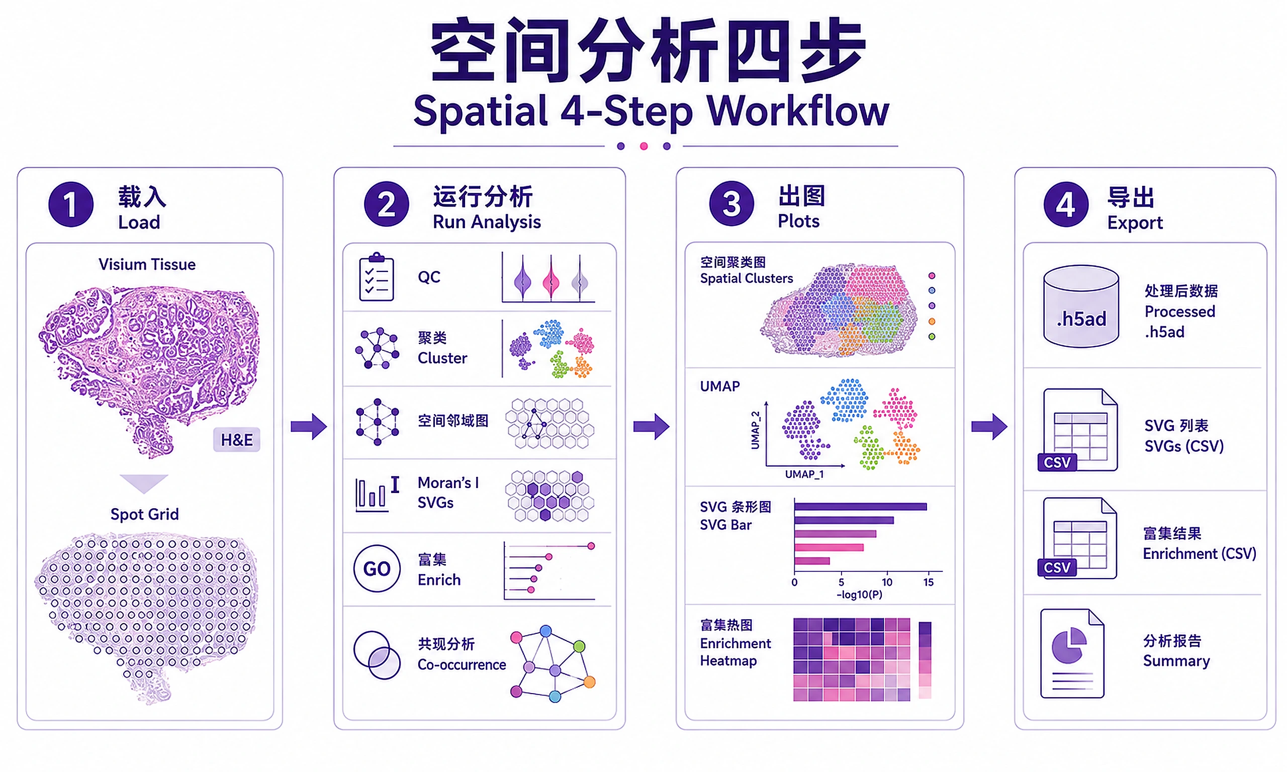
Standard Workflow
🚨 MANDATORY: USE SCRIPTS EXACTLY AS SHOWN — DO NOT WRITE INLINE CODE 🚨
Note: Run from the
spatial-transcriptomics/directory, or addscripts/tosys.path:python import sys; sys.path.insert(0, 'scripts')
Step 1 — Load data:
from load_example_data import load_visium_heart
adata = load_visium_heart()
DO NOT write inline data loading code. Just use the script.
✅ VERIFICATION: You MUST see: "✓ Data loaded successfully!"
Step 2 — Run analysis:
from spatial_workflow import run_spatial_analysis
adata = run_spatial_analysis(adata, output_dir="visium_results")
DO NOT write inline analysis code. Just use the script.
✅ VERIFICATION: You MUST see: "✓ Spatial analysis completed successfully!"
❌ IF YOU DON'T SEE THIS: You wrote inline code. Stop and use the script.
Step 3 — Generate visualizations:
from generate_all_plots import generate_all_plots
generate_all_plots(adata, output_dir="visium_results")
# For non-cardiac tissue, pass tissue-appropriate markers:
# generate_all_plots(adata, output_dir="visium_results", marker_genes=["GENE1", "GENE2"])
DO NOT write inline plotting code (plt.savefig, ggplot, clustermap, etc.). Just use the script.
The script handles PNG + SVG export with graceful fallback for SVG.
✅ VERIFICATION: You MUST see: "✓ All visualizations generated successfully!"
Step 4 — Export results:
from export_results import export_all
export_all(adata, output_dir="visium_results")
DO NOT write custom export code. Use export_all().
✅ VERIFICATION: You MUST see:
==================================================
=== Export Complete ===
==================================================
⚠️ CRITICAL — DO NOT:
- ❌ Write inline analysis code → STOP: Use
run_spatial_analysis() - ❌ Write inline plotting code → STOP: Use
generate_all_plots() - ❌ Write custom export code → STOP: Use
export_all() - ❌ Try to install system libraries → scripts handle optional deps gracefully
⚠️ IF SCRIPTS FAIL — Script Failure Hierarchy:
- Fix and Retry (90%) — Install missing package, re-run script
- Modify Script (5%) — Edit the script file itself, document changes
- Use as Reference (4%) — Read script, adapt approach, cite source
- Write from Scratch (1%) — Only if genuinely impossible, explain why
NEVER skip directly to writing inline code without trying the script first.
Common Issues
| Error | Cause | Fix |
|---|---|---|
ModuleNotFoundError: squidpy |
Missing package | pip install squidpy |
ModuleNotFoundError: plotnine_prism |
Missing theme package | pip install plotnine-prism |
| SVG export failed | Missing SVG backend | Normal — PNG always generated. SVG is best-effort. |
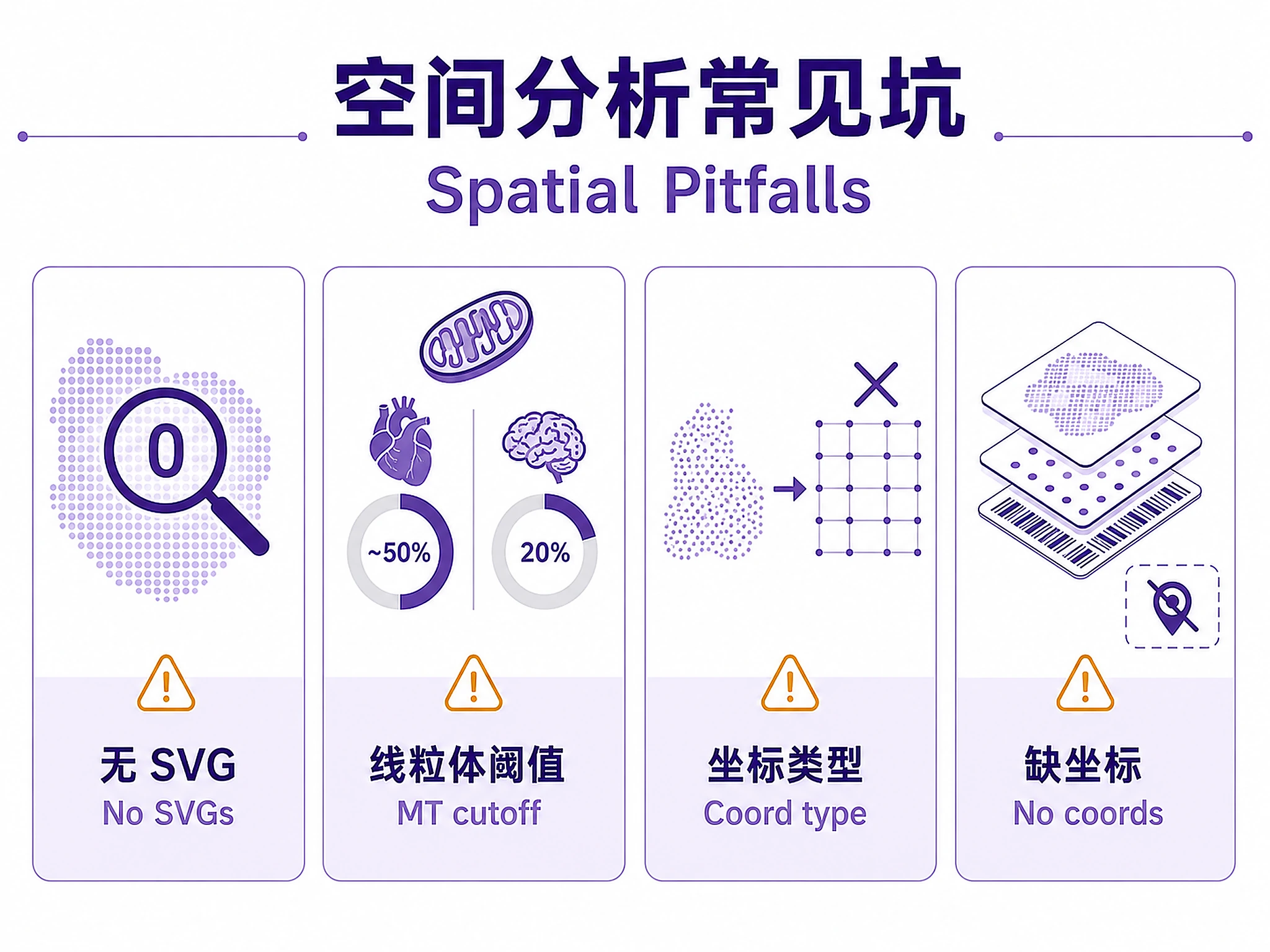
ValueError: coord_type='grid' |
Non-grid spatial data | Use coord_type='generic' for non-Visium data |
| 0 SVGs found (FDR < 0.05) | Low signal or few permutations | Increase svgs_n_perms=1000 or relax FDR threshold |
| Memory error on large dataset | Too many spots/genes | Filter more aggressively or use sc.pp.subsample() |
KeyError: 'spatial' |
Missing spatial coordinates | Ensure data was loaded with sc.read_visium() or has .obsm['spatial'] |
| NaN in co-occurrence | Known squidpy issue with n_splits |
Use default n_splits parameter (do not override) |
Interpreting Results
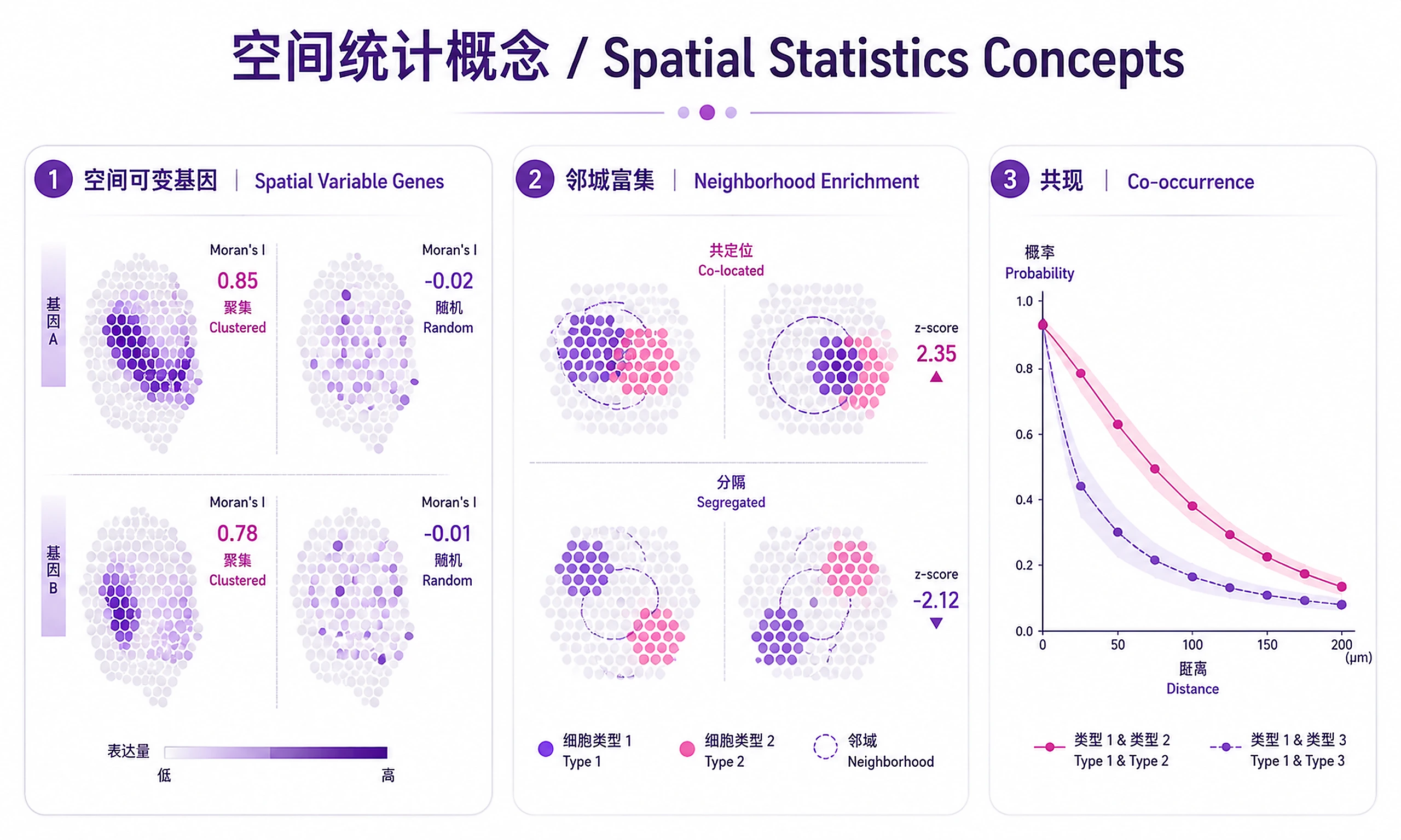
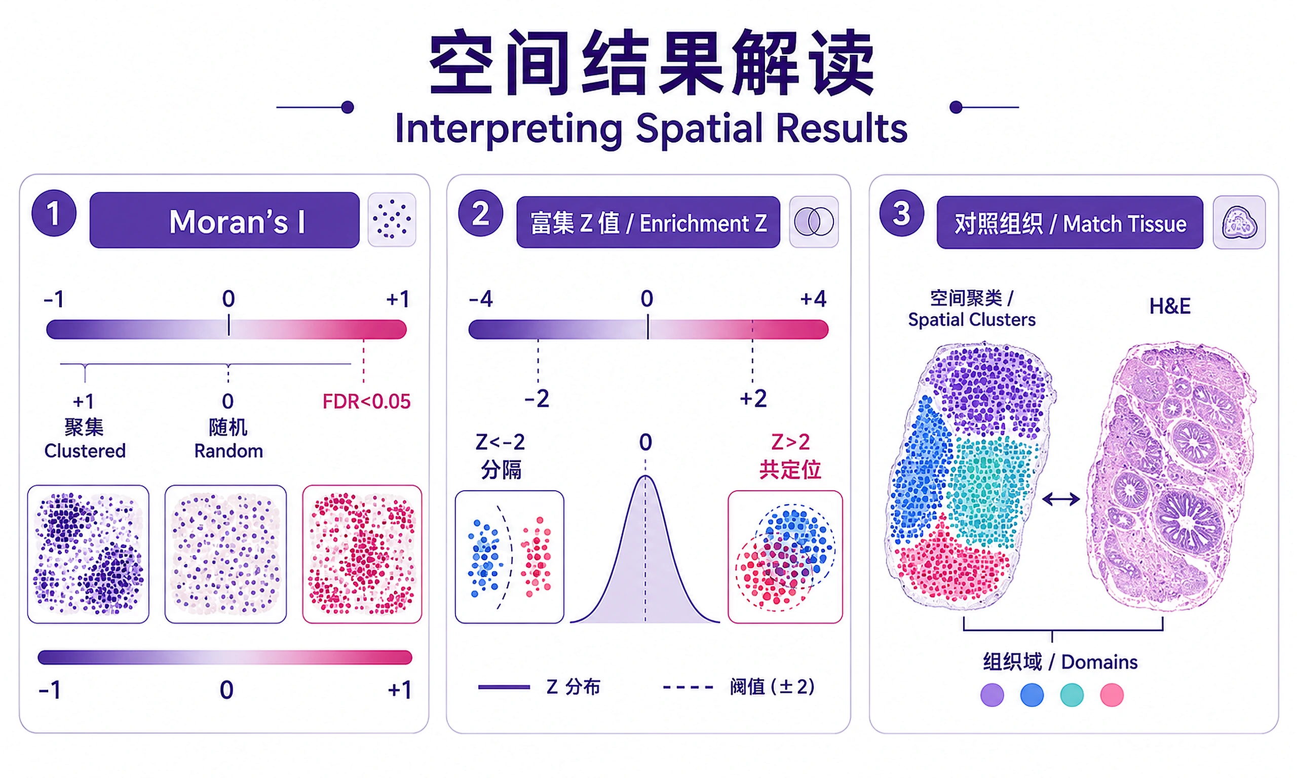
Spatially Variable Genes (SVGs):
- Moran's I close to +1 → Gene expression is spatially clustered (strong spatial pattern)
- Moran's I close to 0 → No spatial structure (random distribution)
- Moran's I close to -1 → Dispersed pattern (checkerboard; rare in practice)
- FDR < 0.05 is the standard significance threshold; use < 0.01 for stringent filtering
- Top SVGs typically include tissue-specific markers and boundary genes
Neighborhood Enrichment Z-scores:
- Z > 2 → Clusters are significantly co-localized (tend to be spatially adjacent)
- Z < -2 → Clusters are significantly segregated (avoid each other spatially)
- -2 to 2 → No significant spatial preference
- Diagonal values (self-enrichment) indicate how spatially cohesive each cluster is
Co-occurrence Curves:
- Probability above expected → Clusters co-occur more than random at that distance
- Distance-dependent changes reveal spatial organization (e.g., border zone cell types co-occur at short range)
Cluster-to-Tissue Mapping:
- Compare spatial cluster plots with H&E histology to validate biological relevance
- Well-defined spatial clusters that match visible tissue structures (e.g., myocardium, fibrotic region) indicate meaningful tissue domains
Agent Summary Guidelines
When presenting results to the user, the agent should:
- Report key numbers: spots analyzed, clusters found, number of significant SVGs
- Highlight top 5-10 SVGs with Moran's I values and known biological roles
- Describe spatial patterns: which clusters are co-localized vs segregated
- Connect to biology: relate spatial patterns to tissue architecture visible in H&E
- Note limitations: permutation count affects SVG p-values; low
n_permsmay miss weak signals - DO NOT hallucinate gene functions — only report known annotations or suggest looking up unknown genes
- DO NOT over-interpret co-occurrence curves from small datasets or few clusters
Mitochondrial content note: Cardiac/muscle tissue has naturally high MT% (~30-40%) due to mitochondria-rich cells. The default max_pct_mito=50% is appropriate for heart tissue. For other tissues (brain, liver, immune), use 20% or lower.
Suggested Next Steps
- Functional enrichment on SVG gene sets →
functional-enrichment-from-degs - Cell type deconvolution with cell2location or RCTD (specialized workflow)
- Cell-cell communication with CellChat or COMMOT on spatial data
- Multi-sample integration for comparing conditions (e.g., MI vs healthy)
- Gene regulatory networks on spatial clusters →
grn-pyscenic
Related Skills
| Skill | Relationship |
|---|---|
scrnaseq-scanpy-core-analysis |
Companion scRNA-seq analysis (non-spatial) |
functional-enrichment-from-degs |
Downstream: enrichment on SVG gene lists |
de-results-to-gene-lists |
Downstream: gene list preparation from SVGs |
grn-pyscenic |
Downstream: regulatory networks from spatial clusters |
coexpression-network |
Downstream: co-expression on spatial domains |
References
- Squidpy: Palla G, et al. "Squidpy: a scalable framework for spatial omics analysis." Nature Methods (2022). doi:10.1038/s41592-021-01358-2
- Scanpy: Wolf FA, et al. "SCANPY: large-scale single-cell gene expression data analysis." Genome Biology (2018). doi:10.1186/s13059-017-1382-0
- Moran's I: Moran PAP. "Notes on continuous stochastic phenomena." Biometrika (1950). doi:10.2307/2332142
- 10x Visium: 10x Genomics. "Visium Spatial Gene Expression." https://www.10xgenomics.com/platforms/visium
Detailed parameter guidance: See references/spatial-analysis-guide.md
Code preview
scripts/export_results.py
"""
============================================================================
EXPORT SPATIAL ANALYSIS RESULTS
============================================================================

Functions:
  - export_all(): Export all results from spatial analysis

Usage:
  from export_results import export_all
  export_all(adata, output_dir="visium_results")
"""

import os
import numpy as np
import pandas as pd
from pathlib import Path
from datetime import datetime


def export_all(
    adata: 'anndata.AnnData',
    output_dir: str = "visium_results"
) -> None:
    """
    Export all spatial transcriptomics analysis results.

    Exports:
    1. adata_processed.h5ad — complete processed AnnData (CRITICAL)
    2. spatially_variable_genes.csv — SVGs with Moran's I statistics
    3. cluster_assignments.csv — spot barcodes + cluster + spatial coords
    4. neighborhood_enrichment.csv — cluster-cluster enrichment z-scores
    5. spot_metadata.csv — all obs columns
    6. analysis_summary.txt — human-readable report

    Parameters
    ----------
    adata : AnnData
        Processed AnnData from run_spatial_analysis().
    output_dir : str
        Output directory (default: "visium_results").
    """
    print("\n=== Step 4: Export Results ===\n")

    output_dir = Path(output_dir)
    output_dir.mkdir(parents=True, exist_ok=True)

    # --- 1. Save processed h5ad (CRITICAL for downstream skills) ---
    print("1. Saving processed AnnData object...")
    h5ad_path = output_dir / "adata_processed.h5ad"
    adata_save = adata.copy()
    # Clean uns for h5ad serialization (remove non-serializable objects)
    _clean_uns_for_h5ad(adata_save)
    adata_save.write_h5ad(h5ad_path, compression='gzip')
    file_size_mb = h5ad_path.stat().st_size / (1024 * 1024)
    print(f"   ✓ {h5ad_path} ({file_size_mb:.1f} MB)")
    print(f"   (Load with: adata = sc.read_h5ad('adata_processed.h5ad'))")

    # --- 2. Spatially variable genes ---
    print("\n2. Exporting spatially variable genes...")
    svg_results = adata.uns.get('svg_results', None)
    if svg_results is not None and len(svg_results) > 0:
        svg_path = output_dir / "spatially_variable_genes.csv"
        svg_results.to_csv(svg_path)
        print(f"   ✓ {svg_path} ({len(svg_results)} genes)")
    else:
        print("   (No SVG results to export)")

    # --- 3. Cluster assignments with spatial coordinates ---
    print("\n3. Exporting cluster assignments...")
    cluster_df = pd.DataFrame({
        'barcode': adata.obs_names,
        'cluster': adata.obs['leiden'].values,
        'spatial_x': adata.obsm['spatial'][:, 0],
        'spatial_y': adata.obsm['spatial'][:, 1],
    })
    if 'total_counts' in adata.obs.columns:
        cluster_df['total_counts'] = adata.obs['total_counts'].values
    if 'n_genes_by_counts' in adata.obs.columns:
        cluster_df['n_genes'] = adata.obs['n_genes_by_counts'].values
scripts/generate_all_plots.py
"""
============================================================================
SPATIAL TRANSCRIPTOMICS VISUALIZATION
============================================================================

Generate publication-quality plots for spatial analysis results.
Uses plotnine + theme_prism() for standard plots, seaborn for heatmaps,
and scanpy/squidpy for spatial tissue overlays.

Functions:
  - generate_all_plots(): Generate all visualizations (PNG + SVG)

Usage:
  from generate_all_plots import generate_all_plots
  generate_all_plots(adata, output_dir="visium_results")
"""

import numpy as np
import pandas as pd
import matplotlib
matplotlib.use('Agg')
import matplotlib.pyplot as plt
import seaborn as sns
from pathlib import Path
from typing import Optional, List, Union

from plotnine import (
    ggplot, aes, geom_violin, geom_jitter, geom_point, geom_col,
    geom_line, labs, theme, coord_flip, facet_wrap, element_text,
    element_blank, scale_color_cmap, guides, guide_legend,
    scale_fill_hue, scale_color_hue
)
from plotnine_prism import theme_prism


# ---------------------------------------------------------------------------
# Save helper: PNG + SVG with graceful fallback
# ---------------------------------------------------------------------------

def _save_plot(fig, base_path: Union[str, Path], dpi: int = 300,
               width: float = 8, height: float = 6) -> None:
    """Save plot in PNG + SVG with graceful SVG fallback."""
    base_path = Path(base_path)
    base_no_ext = base_path.with_suffix('')

    # Always save PNG
    png_path = base_no_ext.with_suffix('.png')
    try:
        if hasattr(fig, 'save'):  # plotnine
            fig.save(str(png_path), width=width, height=height, dpi=dpi, verbose=False)
        else:  # matplotlib figure
            fig.savefig(str(png_path), dpi=dpi, bbox_inches='tight', format='png')
        print(f"   Saved: {png_path}")
    except Exception as e:
        print(f"   Warning: PNG export failed: {e}")

    # Always try SVG
    svg_path = base_no_ext.with_suffix('.svg')
    try:
        if hasattr(fig, 'save'):  # plotnine
            fig.save(str(svg_path), width=width, height=height, verbose=False)
        else:  # matplotlib figure
            fig.savefig(str(svg_path), bbox_inches='tight', format='svg')
        print(f"   Saved: {svg_path}")
    except Exception:
        print(f"   (SVG export failed)")


def _save_matplotlib(fig, base_path, dpi=300, width=8, height=6):
    """Save matplotlib figure and close it."""
    _save_plot(fig, base_path, dpi=dpi, width=width, height=height)
    plt.close(fig)


# ---------------------------------------------------------------------------
# Individual plot functions
# ---------------------------------------------------------------------------

def _plot_qc_violins(adata, output_dir: Path) -> None:
    """QC violin plots using plotnine + theme_prism."""
scripts/load_example_data.py
"""
============================================================================
LOAD SPATIAL TRANSCRIPTOMICS DATA
============================================================================

Functions:
  - load_visium_heart(): Load V1_Human_Heart example dataset from 10x Genomics
  - load_visium_data(): Load user-provided Visium data (h5ad or Space Ranger)

Usage:
  from load_example_data import load_visium_heart
  adata = load_visium_heart()
"""

from pathlib import Path
from typing import Optional, Union


def load_visium_heart() -> 'anndata.AnnData':
    """
    Load V1_Human_Heart Visium dataset from 10x Genomics.

    Downloads the processed dataset via scanpy's built-in datasets module.
    Contains ~4,247 spots and ~33,538 genes with H&E tissue image.

    Returns
    -------
    AnnData
        Visium spatial transcriptomics data with:
        - .X: count matrix (spots x genes)
        - .obs: spot metadata
        - .obsm['spatial']: spatial coordinates
        - .uns['spatial']: tissue image and scalefactors
    """
    import scanpy as sc

    print("Loading V1_Human_Heart Visium dataset...")
    print("  Source: 10x Genomics Spatial Gene Expression")
    print("  Description: Human heart tissue section")
    print("  Platform: Visium Spatial Gene Expression")
    print("  (First run downloads ~50 MB, subsequent runs use cache)")

    try:
        adata = sc.datasets.visium_sge(sample_id="V1_Human_Heart")
    except AttributeError:
        # Fallback for Python <3.12 (tarfile.data_filter not available)
        print("  Using manual download fallback...")
        adata = _download_visium_manual("V1_Human_Heart")

    # Make variable names unique (critical for some Visium datasets)
    adata.var_names_make_unique()

    # Report dataset summary
    has_image = 'spatial' in adata.uns and len(adata.uns['spatial']) > 0

    print(f"\n✓ Data loaded successfully!")
    print(f"  Spots: {adata.n_obs}")
    print(f"  Genes: {adata.n_vars}")
    print(f"  Spatial image: {'Yes' if has_image else 'No'}")
    if 'spatial' in adata.obsm:
        print(f"  Spatial coordinates: {adata.obsm['spatial'].shape}")

    return adata


def _download_file(url: str, dest: Path) -> None:
    """Download a file with proper User-Agent header."""
    import urllib.request

    req = urllib.request.Request(url, headers={
        'User-Agent': 'Mozilla/5.0 (compatible; scanpy-downloader)'
    })
    with urllib.request.urlopen(req) as response, open(dest, 'wb') as out:
        while True:
            chunk = response.read(8192)
            if not chunk:
                break
            out.write(chunk)
Companion files
| Type | Path | Bytes |
|---|---|---|
| Markdown | references/spatial-analysis-guide.md | 7,229 |
| Python | scripts/export_results.py | 8,526 |
| Python | scripts/generate_all_plots.py | 13,881 |
| Python | scripts/load_example_data.py | 5,644 |
| Python | scripts/spatial_workflow.py | 7,022 |
| Markdown | SKILL.md | 11,589 |
| JSON | skill.meta.json | 1,589 |